3. Collectives
3.1. Supported reduction operators
This section lists the available reduction operators when running collective operations.
3.1.1. ADD
The ADD operator calculates the sums of the respective operands. When an AllReduce collective operation is executed on the following inputs:
input_replica_0: 01,02,03,04
input_replica_1: 05,06,07,08
the result will be:
output_replica_0: 06,08,10,12
output_replica_1: 06,08,10,12
ADD supports the following Poplar types: FLOAT, HALF, INT, LONG_LONG, UNSIGNED_LONG_LONG.
3.1.2. MEAN
The MEAN operator calculates the average of the respective operands. When an AllReduce collective operation is executed on the following inputs:
input_replica_0: 1.0,2.0,3.0,4.0
input_replica_1: 5.0,6.0,7.0,8.0
the result will be:
output_replica_0: 3.0,4.0,5.0,6.0
output_replica_1: 3.0,4.0,5.0,6.0
MEAN only supports floating point data types: FLOAT and HALF.
3.1.3. MUL
The MUL operator multiplies the respective operands. When an AllReduce collective operation is executed on the following inputs:
input_replica_0: 01,02,03,04
input_replica_1: 05,06,07,08
the result will be:
output_replica_0: 05,12,21,32
output_replica_1: 05,12,21,32
MUL supports the following Poplar types: FLOAT, HALF, INT, LONG_LONG, UNSIGNED_LONG_LONG.
3.1.4. MIN
The MIN operator finds the smallest value of the respective operands. When an AllReduce collective operation is executed on the following inputs:
input_replica_0: 01,02,03,04
input_replica_1: 05,06,07,08
the result will be:
output_replica_0: 01,02,03,04
output_replica_1: 01,02,03,04
MIN supports the following Poplar types: FLOAT, HALF, INT, UNSIGNED_INT, LONG_LONG, UNSIGNED_LONG_LONG.
3.1.5. MAX
The MAX operator finds the smallest value of the respective operands. When an AllReduce collective operation is executed on the following inputs:
input_replica_0: 01,02,03,04
input_replica_1: 05,06,07,08
the result will be:
output_replica_0: 05,06,07,08
output_replica_1: 05,06,07,08
MAX supports the following Poplar types: FLOAT, HALF, INT, UNSIGNED_INT, LONG_LONG, UNSIGNED_LONG_LONG.
3.1.6. SQUARE_ADD
The SQUARE_ADD operator calculates the sum of squares of the respective operands. When an AllReduce collective operation is executed on the following inputs:
input_replica_0: 01,02,03,04
input_replica_1: 05,06,07,08
the result will be:
output_replica_0: 26,40,58,80
output_replica_1: 26,40,58,80
SQUARE_ADD supports the following Poplar types: FLOAT, HALF, INT, UNSIGNED_INT, LONG_LONG, UNSIGNED_LONG_LONG.
3.1.7. LOGICAL_AND
The LOGICAL_AND operator calculates the logical AND of the respective operands. When an AllReduce collective operation is executed on the following inputs:
input_replica_0: true,false,true,false
input_replica_1: false,true,true,false
the result will be:
output_replica_0: false,false,true,false
output_replica_1: false,false,true,false
The only Poplar data type supported by the LOGICAL_AND operator is BOOL.
3.1.8. LOGICAL_OR
The LOGICAL_OR operator calculates the logical OR of the respective operands. When an AllReduce collective operation is executed on the following inputs:
input_replica_0: true,false,true,false
input_replica_1: false,true,true,false
the result will be:
output_replica_0: true,true,true,false
output_replica_1: true,true,true,false
The only Poplar data type supported by the LOGICAL_OR operator is BOOL.
3.2. Collective groups
GCL supports a few kinds of communication groups that describe the IPUs taking part in a particular collective operation.
3.2.1. Orthogonal group
ORTHOGONAL groups consist of replicas of IPUs that are assigned to it orthogonally to the replica ordering in the topology. For example, for 16 replicas (replica index = 0 to 15) and a group size of 4, there will be four groups and they are assigned as shown in Table 3.1 and in Fig. 3.1.
Group |
Replicas |
|---|---|
0 |
0, 4, 8, 12 |
1 |
1, 5, 9, 13 |
2 |
2, 6, 10, 14 |
3 |
3, 7, 11, 15 |
If there are N replicas denoted {0, ... N-1} and the group size is k, then there are m = N/k groups of size k:
{0, m, 2m, ...}, {1, m+1, 2m+1, ...} ... {m-1, 2m-1, ... N-1}
ORTHOGONAL groups can be also expressed in terms of stride. Replicas are assigned to groups with a stride defined by the number of groups where \(number\ of\ groups = \frac{number\ of\ replicas}{group\ size}\).
3.2.2. Consecutive group
A CONSECUTIVE group consists of replicas of IPUs that are assigned to it consecutively with the replica ordering.
Each group has a size equal to the size CommGroup is instantiated with. For
example, for 16 replicas (replica index = 0 to 15) and a group size of 4,
the groups are assigned as shown in Table 3.2 and in Fig. 3.1.
Group |
Replicas |
|---|---|
0 |
0, 1, 2, 3 |
1 |
4, 5, 6, 7 |
2 |
8, 9, 10, 11 |
3 |
12, 13, 14, 15 |
If there are N replicas denoted {0, ... N-1} and the group size is k,
then there are N/k groups of size k:
{0, 1, ... k-1}, {k, ... 2k-1} ... {N-k-1, ... N-1}
3.2.3. All group
The ALL group tells GCL that all the replicas are taking part in the collective operation as single group. An example of such a grouping is shown in Table 3.3 and in Fig. 3.1.
Group |
Replicas |
|---|---|
0 |
0, 1, 2, 3, 4, 5, 6, 7, 8, 9, 10, 11, 12, 13, 14, 15 |
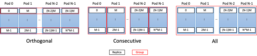
Fig. 3.1 Supported communication groups
3.3. Collective operations
GCL supports the following collective operations:
3.3.1. AllGather
AllGather is an operation where input elements from multiple replicas are distributed to all the participating replicas. For the following inputs:
input_replica_0: [x0,y0]
input_replica_1: [x1,y1]
input_replica_2: [x2,y2]
input_replica_3: [x3,y3]
the result will be:
output_replica_0: [x0,y0,x1,y1,x2,y2,x3,y3]
output_replica_1: [x0,y0,x1,y1,x2,y2,x3,y3]
output_replica_2: [x0,y0,x1,y1,x2,y2,x3,y3]
output_replica_3: [x0,y0,x1,y1,x2,y2,x3,y3]
After the operation, each replica receives the aggregation of data from all replicas in the order of the replicas. The output shape will be calculated as [number_of_input_elements * number_of_replicas]
3.3.2. AllReduce
AllReduce is an operation where input elements are reduced across replicas, with each replica receiving a complete result. For the following inputs:
input_replica_0: x0,y0,z0
input_replica_1: x1,y1,z1
the result will be:
output_replica_0: op(x0,x1),op(y0,y1),op(z0,z1)
output_replica_1: op(x0,x1),op(y0,y1),op(z0,z1)
The output shape will be the same as the input shape and all replicas will have the same data. When ReduceScatter is followed by an AllGather, it becomes equivalent to an AllReduce. In other words, AllReduce(input) == AllGather(ReduceScatter(input)).
3.3.3. AllToAll
AllToAll is an operation where each replica splits its data and sends this split data to all other replicas. The split happens where the split index in the input data matches the index of the recipient’s replica. For the following inputs:
input_replica_0: a0,a1,a2,a3
input_replica_1: b0,b1,b2,b3
input_replica_2: c0,c1,c2,c3
input_replica_3: d0,d1,d2,d3
the result will be:
output_replica_0: a0,b0,c0,d0
output_replica_1: a1,b1,c1,d1
output_replica_2: a2,b2,c2,d2
output_replica_3: a3,b3,c3,d3
The input shape must be equal to the number of replicas in its first dimension (even if it only has one dimension) and the output shape will be equal to the input shape.
3.3.4. Broadcast
Broadcast is an operation where one replica (root replica) will send data to all other replicass. For the following inputs:
 root_replica_0: a0,a1,a2,a3
input_replica_1: b0,b1,b2,b3
input_replica_2: c0,c1,c2,c3
input_replica_3: d0,d1,d2,d3
the result will be:
  root_replica_0: a0,a1,a2,a3
output_replica_1: a0,a1,a2,a3
output_replica_2: a0,a1,a2,a3
output_replica_3: a0,a1,a2,a3
3.3.5. ReduceScatter
ReduceScatter is an operation where input elements are reduced across replicas, with each replica receiving a part of the result. For the following inputs:
input_replica_0: x0,y0,z0
input_replica_1: x1,y1,z1
the result will be:
output_replica_0: op(x0,x1),op(y0,y1)
output_replica_1: op(z0,z1),0
The output shape might not match the input shape as it will be calculated as [ceil(number_of_input_elements / number_of_replicas)].
3.4. Collective methods
This section describes the available collective methods. Collective methods describe the logical network topologies, that is, they define the datapaths in the network.
GCL allows you to control the method selection through the GCL_OPTIONS environment variable described in Section 4.1.1, Option values. The default value for method is auto, which means that GCL will try to pick the optimal method using several variables such as data size, number of replicas in a communication group, communication group type, bytes of data per IPU or physical network topology.
This section describes the collective methods available in GCL.
3.4.1. Anticlockwise ring
This method sends data fragments anticlockwise around the ring of IPUs. The number of fragments is equal to the number of IPUs in the ring.
3.4.2. Bi-directional ring pair
This method splits the data in two and uses the clockwise ring algorithm on one half and the anticlockwise ring algorithm on the other. This will fully use the links in both directions. The number of fragments is equal to twice the number of IPUs in the ring.
3.4.3. Broadcast
This method broadcasts the tensor to all participating replicas in the communication group and performs the reduction locally. This means that the network latency cost is only paid once. This method is faster for small tensors, but comes with a downside of increased memory use if the tensors are larger or the communication group size is too large. There is a GCL_OPTIONS variable that controls this cut-off point after which broadcast will not be selected: syncful.maxBroadcastSize with a default value of 2048 which is group_size * numBytes.
3.4.4. Clockwise ring
This method sends data fragments clockwise around the ring of IPUs. The number of fragments is equal to the number of IPUs in the ring.
3.4.5. Meet-in-the-middle ring
This method sends half of the fragments halfway around the ring in the clockwise direction and half the fragments halfway around the ring in the anticlockwise direction - they meet in the middle. The number of fragments is equal to the number of IPUs in the ring. The disadvantage compared to the bi-directional ring pair method is that the usage of available bandwidth is not quite optimal. In particular, the final step only uses the links in one direction (assuming an even number of IPUs). The advantage is the that this method requires fewer steps and allows the use of larger fragments.
3.4.6. Quad-directional ring
This method divides the fragments in four parts and sends each quarter around one of two rings using the mirrored and non-mirrored ring patterns.