2. Programming with Poplar
You can use Poplar library functions to define graph operations and control the execution and profiling of code on the IPU.
Code can be compiled to run on IPU hardware, a simulated IPU Model or the host CPU. Running on an IPU Model or the CPU may be useful for functional testing of simple code when you do not have access to IPU hardware.
The IPU Model is a simulation of the behaviour of the IPU hardware. It does not completely implement every aspect of a real IPU. For example:
The IPU Model does not fully support replicated graphs (see Replicated graphs).
The arithmetic results may differ from what would be obtained by using the IPU hardware.
Random number generation in the IPU Model is not the same as the hardware. In particular, every simulated tile has the same hard-coded seed (the
setSeed()function is a no op). This means all IPU Model codelets will produce the same results every time they are run. Therefore, the IPU Model should not be used to verify any training or accuracy if the graph includes any random number generation.
If you encounter an out of memory error, it may be useful to run on the IPU Model device to debug the problem.
Consider the situation in which the event trace is being used to investigate a graph that creates a tile memory imbalance. In this case, running on the IPU will lead to an out of memory exception before the report is generated. Running on the IPU Model instead of actual hardware will still run out of memory, but the code will run to completion so the report can be generated.
Code running on a CPU device will be faster than the IPU Model, because it does not have the overhead of modelling the IPU hardware. CPU code runs with a single worker thread as if on a single tile on a single IPU. This means you do not need to think about tile allocation or the limited tile memory when initially developing vertex code. Running on a CPU device may also be useful for unit testing of vertices.
Interrogating a CPU device by calling Engine functions such as
getBytesPerTile() or getTileClockFrequency() may not return accurate or
meaningful results.
If you want to profile your code, you will need to run on either IPU hardware or the IPU Model.
2.1. Poplar programming model
For a more detailed introduction to the IPU architecture and programming model, see the IPU Programmer’s Guide.
A Poplar computation graph defines the input/output relationship between variables and operations. Each variable is a multi-dimensional tensor of typed values and can be distributed across multiple tiles.
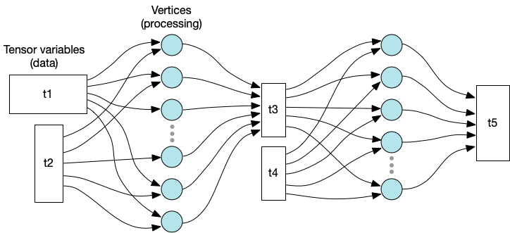
Fig. 2.1 Graph representation of variables and processing
The vertices of the graph are the code executed in parallel by the tiles. Each tile executes a sequence of steps, which form a compute set containing one or more vertices.
The edges of the graph define the data that is read and written by the vertices. Each tile only has direct access to the tensor elements that are stored locally.
Each vertex always reads and writes the same tensor elements. In other words, the connections defined by the execution graph are static and cannot be changed at run time. However, the host program can calculate the mapping and graph connectivity at run time when it constructs the execution graph. See Poplar tutorial 7 on the Graphcore GitHub for an example.
The placement of vertices and tensor elements onto tiles is known as the tile mapping.
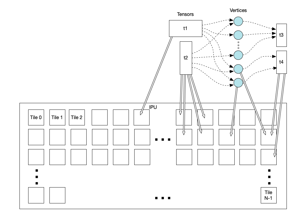
Fig. 2.2 Mapping tensors and vertices to tiles
2.2. The structure of a Poplar program
A Poplar program performs the following tasks:
Find or create the target device type as a
Devicerepresenting physical IPU hardware or a simulatedIPUModel.Create a
Graphobject which will define the connections between computation operations and data, and how they are mapped onto the IPUs.Create one or more
Programobjects which will control the execution of the graph operations.Define the computations to be performed and add them to the
GraphandProgramobjects. You can use the functions defined in Poplar and PopLibs, or you can write your own device code.Create an
Engineobject, which represents a session on the target device, using theGraphandProgramobjects.Connect input and output streams to the
Engineobject, to allow data to be transferred to and from the host.Execute the computation with the
Engineobject. This will compile your graph code and load it onto the IPU, along with any library functions required, and start execution.
A program object can be constructed by combining other program objects in various ways.
For example, Poplar provides several standard Program sub-classes such as Sequence,
which executes a sequence of sub-programs, Repeat for executing loops, and If
for conditional execution.
The Poplar and PopLibs libraries also include programs for a wide range of operations on tensor data.
For more detailed descriptions and examples of each of these steps, see the tutorials on the Graphcore GitHub.
2.2.1. What happens at run time
When you run your program on the host, the Poplar run-time will compile your graph to create object code for each tile. The code may come from Poplar or PopLibs library functions, or from vertex code you write yourself (see Device code), and will be linked with any required libraries.
This object will contain:
The control-program code from your graph
Code to manage exchange sequences
Initialised vertex data
The tensor data mapped to that tile
The host program will load the object code onto the target device, which is then ready to execute the program.
2.3. Virtual graphs
A graph is created for a target device with a specific number of tiles. It is possible to create a new graph from that, which is a virtual graph for a subset of the tiles. This is effectively a new view onto the parent graph for a virtual target, which has a subset of the real target’s tiles and can be treated like a new graph. You can add vertices and tensors to the virtual sub-graphs. These will also appear in the parent graph.
Any change made to the parent graph, such as adding variables or vertices, may also affect the virtual sub-graph. For example, a variable added to the parent graph will appear in the sub-graph if it is mapped to tiles that are within the subset of tiles in the virtual target.
Virtual graphs can be used to manage the assignment of operations to a subset of the available tiles. This can be used, for example, to implement a pipeline of operations by creating a virtual graph for each stage of the pipeline and adding the operations to be performed on those tiles.
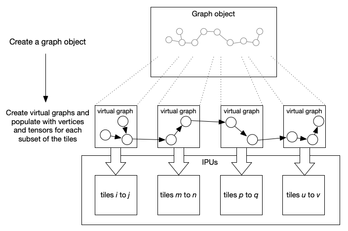
Fig. 2.3 Mapping a pipeline of operations to tiles using virtual graphs
There are several versions of the createVirtualGraph function, which
provide different ways of selecting the subset of tiles to include in the
virtual target.
2.4. Replicated graphs
You can also create a replicated graph. This effectively creates a number of identical copies, or replicas, of the same graph. Each replica targets a different subset of the available tiles (all subsets are the same size). This may be useful, for example, where the target consists of multiple IPUs and you want to create a replica to run on each IPU (or group of IPUs) in parallel.
Any change made to the replicated graph, such as adding variables or vertices, will affect all the replicas. A variable mapped to tile 0, for example, will have an instance on tile 0 in each of the replicas.
Replicated graphs can be created in two ways:
Splitting an existing graph into a number replicas with the
createReplicatedGraphfunction (see Replicating an existing graph).Creating a new replicated top-level graph by passing a replication factor to the
Graphconstructor (see Creating a replicated graph).Note: Replicated graphs created in this way are not supported when running on an IPU Model.
As an example, imagine you have a graph which targets two IPUs. You can run four copies of it, in parallel, on eight of the IPUs in your system by creating the two-IPU graph and replicating it four times. This can be done using either of the techniques above, each of which has advantages and disadvantages, summarised in the following descriptions.
2.4.1. Replicating an existing graph
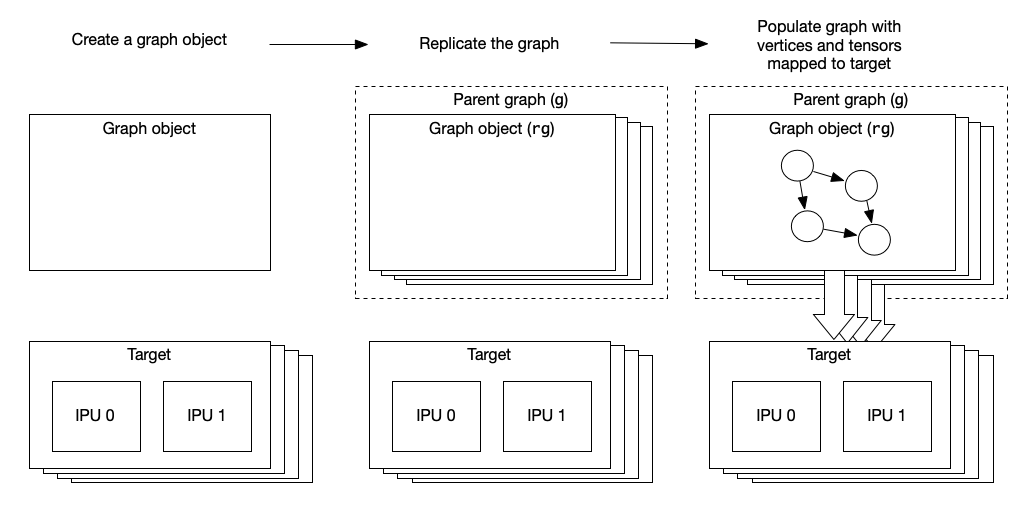
Fig. 2.4 Replicating an existing graph
We can start by creating a graph for eight IPUs, and then creating a replicated graph from that:
// Create a graph for 'target' which has 8 IPUs
Graph g  = Graph(target);
// Create 4 replicas each of which targets 2 IPUs
Graph rg = g.createReplicatedGraph(4);
Any changes, such as adding code or variables, made to the replica rg will
be duplicated over all four replicas.
However, you can still do things with the original “parent” graph g that do not affect all the replicas. For example, a variable or an operation can be added to the parent graph and mapped to only one IPU. This will only be present on the replica that targets that IPU. It is also possible to access a variable that exists on all the replicas as a single tensor, using the getNonReplicatedTensor function. This adds an extra dimension to the variable to represent the mapping across the replicas.
This approach provides more flexibility but means that the graph of each replica needs to be compiled separately. This can make it slower to build the program.
2.4.2. Creating a replicated graph
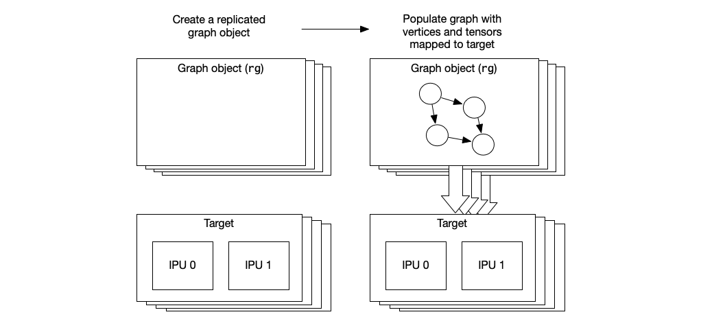
Fig. 2.5 Creating a replicated graph
In this case, we start by creating a replicated graph using the graph constructor:
// Create a graph with 4 replicas for each 2 IPUs
Graph rg = Graph(target, replication_factor(4));
We can add variables and vertices to this graph as usual. These additions will
be applied to every replica. This graph only exists as a replica, with no
parent graph that can be used to make modifications differently to each
replica. Therefore, as all the replicas are guaranteed to be identical, the
graph only needs to be compiled once. Copies of the object code are then loaded
onto each of the pairs of IPUs when the program runs. Each instance of the
replica is given a unique ID at load time; this can be used to identify it in
functions such as crossReplicaCopy.
Any functions that rely on the existence of a parent, such as getTopLevelGraph or getNonReplicatedTensor, will fail.
2.5. Data streams and remote buffers
Memory external to the IPU can be accessed in two ways. Data streams enable the IPU to transfer data to and from host memory. Remote buffers enable the IPU to store data in external (off-chip) memory.
2.5.1. Data streams
Data streams are used for communication between the host and the IPU device. The data transfers are controlled by the IPU.
Each stream is a unidirectional communication from the host to the device, or from the device to the host. A stream is defined to transfer a specific number of elements of a given type. This means the buffer storage required by the stream is known (the size of the data elements times the number of elements).
The Poplar graph compiler will merge multiple stream transfers into a single transfer (up to the limits described in Stream buffer size limit).
Device-side streams
A stream object, represented by the DataStream class, is created and added to a graph using the addHostToDeviceFIFO or addDeviceToHostFIFO functions.
The stream is defined to have:
A name for the stream
The type of data to be transferred
The number of elements to be transferred
A host-to-device stream can also have a replication mode, if it is connected to a replicated graph. This defines whether a single stream will send the same data to all the replicated graphs (broadcast mode) or there will be a stream per replica.
Stream data transfer is done with a Copy program which copies data from the stream to a tensor, or from a tensor to the stream.
Host-side stream access
On the host side, a data stream is connected to a buffer allocated in memory. The buffer is connected to the stream using the connectStream function of an Engine object. This can, optionally, be implemented as a circular buffer to support more flexible transfers.
In order to synchronise with the data transfers from the IPU, a callback is
connected to the stream using the Engine::connectStreamToCallback function.
Callback implementations are derived from the StreamCallback interface and
have a pointer to the stream buffer as an argument.
For a device-to-host transfer, the callback function will be called when the transfer is complete so that the host can read the data from the buffer.
For a host-to-device stream, by default the callback function will be called immediately before the IPU transfers the buffer contents to device memory. The host-side code should populate the stream buffer and then return.
2.5.2. Optimising host data transfers
There are several things you can do to optimise the use of data streams to and from the host. These are described below.
Prefetch
You can specify that the the IPU should call the callback function as early as possible (for example, immediately after it releases the stream buffer from a previous transfer). The host is then able to fill the buffer in advance of the transfer, meaning the IPU spends less time waiting for the host.
This mode of operation, known as prefetch, is enabled by setting the
exchange.enablePrefetch option to “true” when the engine object is created.
Prefetch is only possible if the address range of the stream’s data buffer does not overlap with another stream’s buffer (this may be done to optimise memory use).
This means that the engine option exchange.streamBufferOverlap
must be set to either “HostRearrangeOnly” or “None”. The first of these is most
useful as the performance of streams that are being rearranged is often
less important. Setting the option to “None” may use too much memory.
The callback function returns a value that indicates if the buffer was filled.
If there is data available to fill the buffer, the callback function should
return Result::Success. The device code will then call the complete
callback when it has transferred the data.
Otherwise, if data is not available (either because it is the end of the
stream, or the data is not ready yet), then the callback returns
Result::NotAvailable.
IPU-Link and sync configuration
Multiple IPUs can be connected with IPU-Links to share data. There are also synchronisation (sync) signals that are used to indicate when IPUs are ready to exchange data and that data exchange is complete. These sync signals are also used to synchronise host transfers and access to remote buffers.
Link topologies
There are two ways of connecting IPU-Links and sync signals: in a mesh or as a torus. The mesh structure is similar to a ladder, where pairs of IPUs form each rung. In a torus, the ends of the “ladder” loop round to form a closed loop.
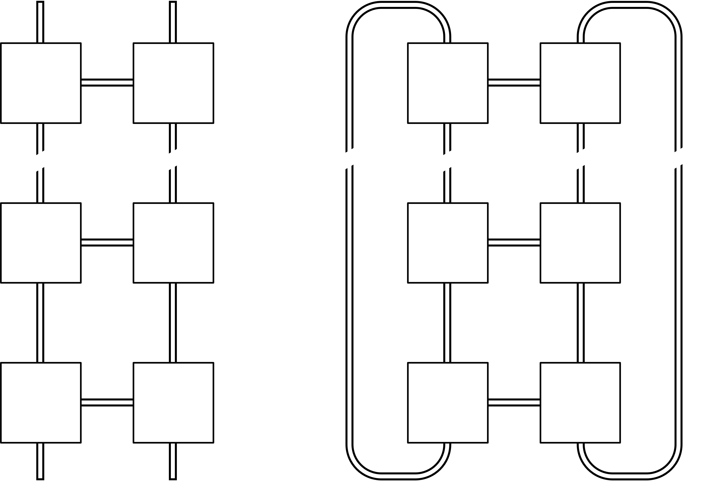
Fig. 2.6 Mesh and torus link topologies
When a target device is created in a Poplar program, the topology is defined by
the ipuLinkTopology option to the Target object.
Sync groups
Each IPU can be allocated to one or more “sync groups”. At a synchronization point, all the IPUs in a sync group will wait until all the other IPUs in the group are ready.
Sync groups can be used to to allow subsets of IPUs to overlap their operations. For example, one sync group can be performing data transfers to or from the host, while another group is processing a previous batch of data.
You can configure the sync groups as appropriate for your application. The allocation
of IPUs to the sync groups (GS1 and GS2) can be configured using the syncConfiguration option
when creating a target.
The options are:
intraReplicaAndAll:
GS1 is used for synchronisation between the IPUs in each replica of a replicated graph (or all IPUs if there is no replication).
GS2 is used for synchronisation between all IPUs.
ipuAndAll:
GS1 is used for synchronisation of each IPU individually.
GS2 is used for synchronisation between all IPUs.
intraReplicaAndLadder:
GS1 is used for synchronisation between the IPUs in each replica of a replicated graph (or all IPUs if there is no replication).
GS2 is used by two independent subsets of IPUs. These can then synchronise independently of one another, so that they can alternate between one set doing host I/O, for example, while the other is computing.
The way in which Poplar uses these sync groups is summarised in the following table:
syncConfiguration |
syncReplicasIndependently |
||
|---|---|---|---|
false (default) |
true |
||
intraReplicaAndAll (default) and intraReplicaAndLadder |
GS1 |
Communication between IPUs within each replica (or all IPUs if the graph is not replicated). Remote buffer access. |
Communication between IPUs within each replica (or all IPUs if the graph is not replicated). Remote buffer access. Host communication. |
GS2 |
Communication between replicas (all IPUs). Host communication. |
Communication between replicas (all IPUs). |
|
ipuAndAll |
GS1 |
Remote buffer access. |
Remote buffer access. Host communication. |
GS2 |
Communication between all IPUs. Host communication. |
Communication between all IPUs. |
|
Software sync
Software sync provides a third synchronisation mechanism that can replace the
hardware sync that happens after a host exchange. Software sync is disabled by
default. You can enable it by setting the option opt.enableSwSyncs to true
when creating the engine object.
With software sync enabled, each IPU synchronises with the host independently. This means that each IPU can move onto the next operation as soon as its host data transfer is complete, instead of having to wait for all the other IPUs to finish.
If two IPUs don’t need to synchronise then they can operate in parallel, completely independently. For example, this allows one to do I/O while the other is computing. But this applies more generally: each IPU can do an arbitrary sequence of compute and I/O operations without needing to synchronise with the other IPU until they need to communicate with one another.
Note
If you use software sync then the default sync configuration
(intraReplicaAndAll) must be used and the
target.syncReplicasIndependently option must not be set.
2.5.3. Remote memory buffers
The IPU can also access off-chip memory as a remote buffer. This may be host memory or memory associated with the IPU system. This is not used for transferring data to the host, but just for data storage by the IPU program.
A RemoteBuffer object is created and added to the graph with the addRemoteBuffer function of the graph object. Data transfers to and from the remote buffer are performed using a Copy program which copies data from the buffer to a tensor, or from a tensor to the buffer.
The data type and size of the remote buffer are defined when it is created.
The definition of the buffer and the parameters to the Copy program allow
for very flexible addressing.
You can think of the buffer containing a number of data transfer “rows” of data. (These rows do not need to correspond to the structure the tensor being transferred or the organisation of the data in the buffer, but are just a way of managing data transfers.)
The size of each row and the number of rows are parameters to
addRemoteBuffer when the buffer is created. Each row contains
numElements data items and the entire buffer contains repeat rows.
Each transfer to or from the remote buffer can copy one or more rows of data.
The rows to be copied are specified by the offset parameter to the Copy
program. The number of offsets specifies the number of rows to copy.
2.5.4. Stream buffer size limit
The IPU has a memory address translation table which defines the external memory address range it can access. As a result, there is a maximum buffer size for data transferred by a stream. This limit is currently 128 MBytes per stream copy operation. More data can be transferred by a sequence of copies, separated by sync operations, so that the buffer memory can be reused for each transfer.
Each IPU has its own translation table. So, if there are multiple IPUs, this limit applies to each IPU individually.
2.6. Device code
Each vertex of the graph is associated with some device code. This can come from a library function or you can write your own as a codelet. Codelets are specified as a class that inherits from the poplar::Vertex type. For example:
#include <poplar/Vertex.hpp>

using namespace poplar;

class AdderVertex : public Vertex {
public:
  Input<float> x;
  Input<float> y;
  Output<float> sum;

  bool compute() {
    *sum = x + y;
    return true;
  }
};
The Input and Output fields connect the vertex to the tensor data that
it reads and writes. An Input field should not be written and an Output
field should not be read; the results are undefined. If you need a field that
is read and written, then it should be defined as InOut.
These fields have begin, end, operator[] and operator* methods
so they can be iterated over and accessed like other C++ containers.
For Input fields all of these methods are const.
The Output field can be successfully updated even if the corresponding
tensor is on another tile. This is because the data is not transferred to the
destination tile until the compute is complete. However, reading an
Output field is not guaranteed to return the expected value. If you need to
both write to and read from a field, then it should be declared as an InOut
type.
The types used in vertex code are described in the runtime API section of the Poplar and PopLibs API Reference.
You can add a codelet to your graph by using the Graph::addCodelets
function. This will load the source file and compile the codelet when the host
program runs. See the adder example provided with the Poplar
distribution.
You can also pass compilation options (for example “-O3”). The code is compiled for both the host and for the IPU so the program can be run on IPU hardware or on the host.
There are a couple of predefined macros that may be useful when writing vertex code. __POPC__ is defined when code is compiled by the codelet compiler. The macro __IPU__ is defined when code is being compiled for the IPU (rather than the host).
You can also write codelets in assembly language for the IPU. See the Vertex Assembly Programming Guide for more information. You might find that document useful even if you are not programming in assembly, as it contains a lot of information about calling conventions, memory use and the implementation of various data structures.
2.6.1. Stack allocation
When C++ functions are compiled, the compiler is usually able to determine the stack required. This is not possible if you use recursion, function calls via pointers or variable-length arrays (array variables that have a size that is not a compile time constant).
If you must use these techniques, then you must explicitly specify the stack
used by your functions. Macros are provided for this purpose. These
are defined in the Poplar header file StackSizeDefs.hpp.
See the runtime API section of the
Poplar API Reference
for more information.
DEF_STACK_USAGE size functionThis defines the total stack usage (in bytes) for the function specified and any functions that it calls. This means that Poplar will not traverse the call graph of the function to determine the total stack usage of the function.
If you use recursion, this macro must be used to specify the total stack usage of the recursive function itself, taking into account the maximum depth of the recursion and any other functions that can be called.
DEF_FUNC_CALL_PTRSThis defines a list of other functions that may be called via pointers. Note that this creates a maintainability problem as the macro use must be updated every time the code changes its use of function pointers.
2.6.2. Pre-compiling codelets
There is a command line tool to pre-compile codelets. This reduces loading time, and allows you to check for errors before running the host program.
The codelet compiler, popc, takes your source code as input and creates a
graph program object file (conventionally, with a .gp file extension). For
example:
$ popc codelets.cpp -o codelets.gp
This object file can be added to your graph in the same way as source codelets,
using the same Graph::addCodelets function. See the adder_popc example
provided with the Poplar distribution.
The general form of the popc command is:
$ popc [options] <input file> -o <output file>
The command takes several command line options. Most are similar to any other C compiler. For example:
-D<macro> |
Add a macro definition |
-I<path> |
Add a directory to the include search path |
-g |
Enable debugging |
-On |
Set the optimization level (n = 0 to 3) |
For a full list of options, use the --help option.