5. Training a model
TensorFlow XLA and Poplar provide the ability to combine an entire training graph into a single operation in the TensorFlow graph. This accelerates training by removing the need to make calls to the IPU hardware for each operation in the graph.
However, if the Python code with the training pass is called multiple times, once for each batch in the training data set, then there is still the overhead of calling the hardware for each batch.
The Graphcore IPU support for TensorFlow provides three mechanisms to improve the training performance: training loops, data set feeds, and replicated graphs.
5.1. Training loops, data sets and feed queues
By placing the training operations inside a loop, they can be executed multiple
times without returning control to the host. It is possible to use a standard
TensorFlow while_loop operation to wrap the training operation, but the IPU
library provides a convenient and feature rich version.
Normally when TensorFlow runs, operations which are not inside a loop will be executed once, and those operations will return one or more tensors with fixed values. However, when a training operation is placed into a loop, the inputs to that training operation need to provide a stream of values. Standard TensorFlow Python feed dictionaries cannot provide data in this form, so when training in a loop, data must be fed from a TensorFlow DataSet.
You can find more information about the DataSet class and its use in normal operation on the TensorFlow Better performance with the tf.data API web page. TensorFlow provides many pre-configured DataSets for use in training models, see TensorFlow Datasets for more information.
To construct a system that will train in a loop, you will need to do the following:
Wrap your optimiser training operation in a loop.
Create an
IPUInfeedQueueto feed data to that loop.Create an
IPUOutfeedQueueto take results out of that loop.Create a TensorFlow DataSet to provide data to the input queue.
The following example shows how to construct a trivial DataSet, attach it to
a model using in IPUInfeedQueue, feed results into an IPUOutfeedQueue, and
construct a loop.
 1from tensorflow.python.ipu import ipu_compiler
 2from tensorflow.python.ipu import ipu_infeed_queue
 3from tensorflow.python.ipu import ipu_outfeed_queue
 4from tensorflow.python.ipu import loops
 5from tensorflow.python.ipu import scopes
 6from tensorflow.python.ipu.config import IPUConfig
 7import tensorflow.compat.v1 as tf
 8tf.disable_v2_behavior()
 9
10# The dataset for feeding the graphs
11ds = tf.data.Dataset.from_tensors(tf.constant(1.0, shape=[800]))
12ds = ds.map(lambda x: [x, x])
13ds = ds.repeat()
14
15# The host side queues
16infeed_queue = ipu_infeed_queue.IPUInfeedQueue(ds)
17outfeed_queue = ipu_outfeed_queue.IPUOutfeedQueue()
18
19
20# The device side main
21def body(x1, x2):
22  d1 = x1 + x2
23  d2 = x1 - x2
24  outfeed = outfeed_queue.enqueue({'d1': d1, 'd2': d2})
25  return outfeed
26
27
28def my_net():
29  r = loops.repeat(10, body, [], infeed_queue)
30  return r
31
32
33with scopes.ipu_scope('/device:IPU:0'):
34  run_loop = ipu_compiler.compile(my_net, inputs=[])
35
36# The outfeed dequeue has to happen after the outfeed enqueue
37dequeue_outfeed = outfeed_queue.dequeue()
38
39# Configure the hardware
40config = IPUConfig()
41config.auto_select_ipus = 1
42config.configure_ipu_system()
43
44with tf.Session() as sess:
45  sess.run(infeed_queue.initializer)
46
47  sess.run(run_loop)
48  result = sess.run(dequeue_outfeed)
49  print(result)
In this case the DataSet is a trivial one. It constructs a base DataSet from a single TensorFlow constant, and then maps the output of that DataSet into a pair of tensors. It then arranges for the DataSet to be repeated indefinitely.
After the DataSet is constructed, the two data feed queues are constructed. The
IPUInfeedQueue takes the DataSet as a parameter.
The IPUOutfeedQueue has extra options to control how it collects and outputs
the data sent to it. None of these are used in this example.
Now that we have the DataSet and the queues for getting data in and out of the
device-side code, we can construct the device-side part of the model. In this
example, the body function constructs a very simple model, which does not
even have an optimiser. It takes the two data samples which will be provided
by the DataSet, and performs some simple maths on them, and inserts the
results into the output queue.
Typically, in this function, the full ML model would be constructed and a
TensorFlow Optimizer would be used to generate a backward pass and variable
update operations. The returned data would typically be a loss value, or
perhaps nothing at all if all we do is call the training operation.
The my_net function is where the loops.repeat function is called. This
wraps the body function in a loop. It takes as the first parameter the
number of times to execute the operation, in this case 10. It also takes the
function that generated the body of the loop, in this case the function
body, a list of extra parameters to pass to the body, in this case none,
and finally the infeed queue which will feed data into the loop.
Next we create an IPU scope at the top level and call ipu_compiler.compile
passing the my_net function, to create the training loop in the main graph.
The output of the ipu_compiler.compile will be an operation that can be
called to execute the training loop.
Finally, we create an operation which can be used to fetch results from the outfeed queue. Note that it isn’t necessary to use an outfeed queue if you do not wish to receive any per-sample output from the training loop. If all you require is the final value of a tensor, then it can be output normally without the need for a queue.
If you run this example then you will find that the result is a Python
dictionary containing two numpy arrays. The first is the d1 array and
will contain x1 + x2 for each iteration in the loop. The second is the d2
array and will contain x1 - x2 for each iteration in the loop.
See entries in the TensorFlow Python API for more details.
5.2. Accessing outfeed queue results during execution
An IPUOutfeedQueue supports the results being fetched continuously during
the execution of a model. This feature can be used to monitor the performance of
the network, for example to check that the loss is decreasing, or to stream
predictions for an inference model to achieve minimal latency for each sample.
 1from threading import Thread
 2
 3from tensorflow.python.ipu import ipu_compiler
 4from tensorflow.python.ipu import ipu_infeed_queue
 5from tensorflow.python.ipu import ipu_outfeed_queue
 6from tensorflow.python.ipu import loops
 7from tensorflow.python.ipu import scopes
 8from tensorflow.python.ipu.config import IPUConfig
 9from tensorflow.python import keras
10import tensorflow.compat.v1 as tf
11tf.disable_v2_behavior()
12
13# The dataset for feeding the graphs
14ds = tf.data.Dataset.from_tensors(tf.constant(1.0, shape=[2, 20]))
15ds = ds.repeat()
16
17# Host side queues that handle data transfer to and from the device
18infeed_queue = ipu_infeed_queue.IPUInfeedQueue(ds)
19outfeed_queue = ipu_outfeed_queue.IPUOutfeedQueue()
20
21
22# A simple inference step that predicts classes for an image with a model
23# composed of three dense layers and sends the predicted classes from the IPU
24# device to the host using an IPUOutfeedQueue
25def inference_step(image):
26  partial = keras.layers.Dense(256, activation=tf.nn.relu)(image)
27  partial = keras.layers.Dense(128, activation=tf.nn.relu)(partial)
28  logits = keras.layers.Dense(10)(partial)
29  classes = tf.argmax(input=logits, axis=1, output_type=tf.dtypes.int32)
30  # Insert an enqueue op into the graph when inference_step is called
31  outfeed = outfeed_queue.enqueue(classes)
32  return outfeed
33
34
35NUM_ITERATIONS = 100
36
37
38def inference_loop():
39  r = loops.repeat(NUM_ITERATIONS, inference_step, [], infeed_queue)
40  return r
41
42
43# Build the main graph and encapsulate it into an IPU cluster
44with scopes.ipu_scope('/device:IPU:0'):
45  run_loop = ipu_compiler.compile(inference_loop, inputs=[])
46
47# Calling outfeed_queue.dequeue() will insert the dequeue op into the graph.
48# We must do this after we've inserted the enqueue op and in the same graph as
49# the enqueue op. Note that threads have different default graphs, so we call it
50# here to ensure both ops are in the same graph.
51dequeue_outfeed = outfeed_queue.dequeue()
52
53# Configure the hardware
54config = IPUConfig()
55config.auto_select_ipus = 1
56config.configure_ipu_system()
57
58with tf.Session() as sess:
59  sess.run(tf.global_variables_initializer())
60  sess.run(infeed_queue.initializer)
61
62  # Function to continuously execute the dequeue op and print the dequeued data
63  def dequeue():
64    counter = 0
65    # We expect 2*`NUM_ITERATIONS` results because we execute the loop twice
66    while counter != NUM_ITERATIONS * 2:
67      r = sess.run(dequeue_outfeed)
68      # Check if there are any results to process
69      if r.size:
70        # Print the partial results
71        for t in r:
72          print("Step:", counter, "classes:", t)
73          counter += 1
74
75  # Execute the main loop once to compile the program. We must do this before
76  # starting the dequeuing thread, or the TensorFlow runtime will try to dequeue
77  # an outfeed that it doesn't know about
78  sess.run(run_loop)
79
80  # Start a thread that asynchronously continuously dequeues the outfeed
81  dequeue_thread = Thread(target=dequeue)
82  dequeue_thread.start()
83
84  # Run the main loop while the outfeed is being dequeued by the second thread
85  sess.run(run_loop)
86
87  # After main loop execution, wait for the dequeuing thread to finish
88  dequeue_thread.join()
You can also follow this tutorial on using outfeed queues to inspect tensors and return activation and gradient tensors from the Graphcore tutorials repository.
5.3. Replicated graphs
To improve performance, multiple IPUs can be configured to run in a data parallel mode. The graph is said to be replicated across multiple IPUs. See the Poplar and PopLibs User Guide for more background about replicated graphs.
The Graphcore tutorials repository also has a tutorial on using replication in TensorFlow to train a simple model.
5.3.1. Selecting the number of replicas
During system configuration, you specify the number of IPUs for the
TensorFlow device using the auto_select_ipus or select_ipus options on
an IPUConfig instance.
A graph can be sharded across multiple IPUs (model parallelism), and then replicated across IPUs (data parallelism). When specifying the number of IPUs in the system, you must specify a multiple of the number of shards used by the graph.
For instance, if a graph is sharded over two IPUs, and you set the
auto_select_ipus option to eight IPUs, then the graph will be replicated
four times.
5.3.2. Performing parameter updates
Each replica maintains its own copy of the graph, but during training it is important to ensure that the graph parameters are updated so that they are in sync across replicas.
A wrapper for standard TensorFlow optimisers is used to add extra operations to
the parameter update nodes in the graph to average updates across replicas.
See tensorflow.python.ipu.optimizers.CrossReplicaOptimizer.
5.4. Pipelined training
The IPU pipeline API creates a series of computational stages, where the outputs of one stage are the inputs to the next one. These stages are then executed in parallel across multiple IPUs. This approach can be used to split the model where layer(s) are executed on different IPUs.
This improves utilisation of the hardware when a model is too large to fit into a single IPU and must be sharded across multiple IPUs.
Each of the stages is a set of operations, and is described using a Python
function, in much the same way as the ipu.compile takes a function that
describes the graph to compile onto the IPU.
See tensorflow.python.ipu.pipelining_ops.pipeline() for details of the
pipeline operator.
The pipeline API requires data inputs to be provided by a tf.DataSet
source connected via an infeed operation. If you would like per-sample
output, for instance the loss, then this will have to be provided by an outfeed
operation.
The computational stages can be interleaved on the devices in three different
ways as described by the pipeline_schedule parameter. By default the API
will use the PipelineSchedule.Grouped mode (Fig. 5.1), where the forward passes are
grouped together, and the backward passes are grouped together. The main
alternative is the PipelineSchedule.Interleaved mode (Fig. 5.2), where the forward and
backward passes are interleaved, so that fewer activations need to be stored. Additionally, the PipelineSchedule.Sequential mode (Fig. 5.3),
where the pipeline is scheduled in the same way as if it were a sharded model,
may be useful when debugging your model.
For more information on pipelining, refer to the technical note on Model parallelism with TensorFlow: sharding and pipelining.
5.4.1. Grouped scheduling
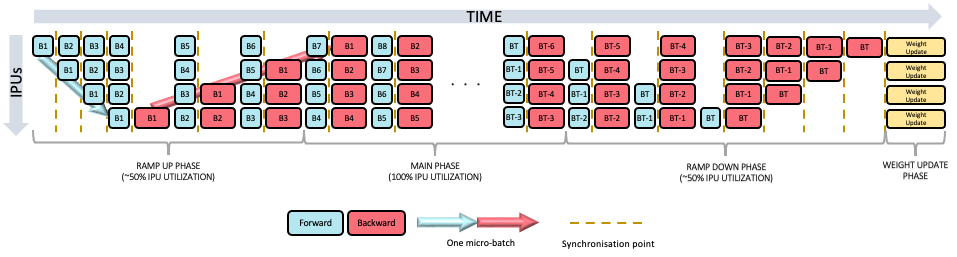
Fig. 5.1 Grouped scheduling
5.4.2. Interleaved scheduling
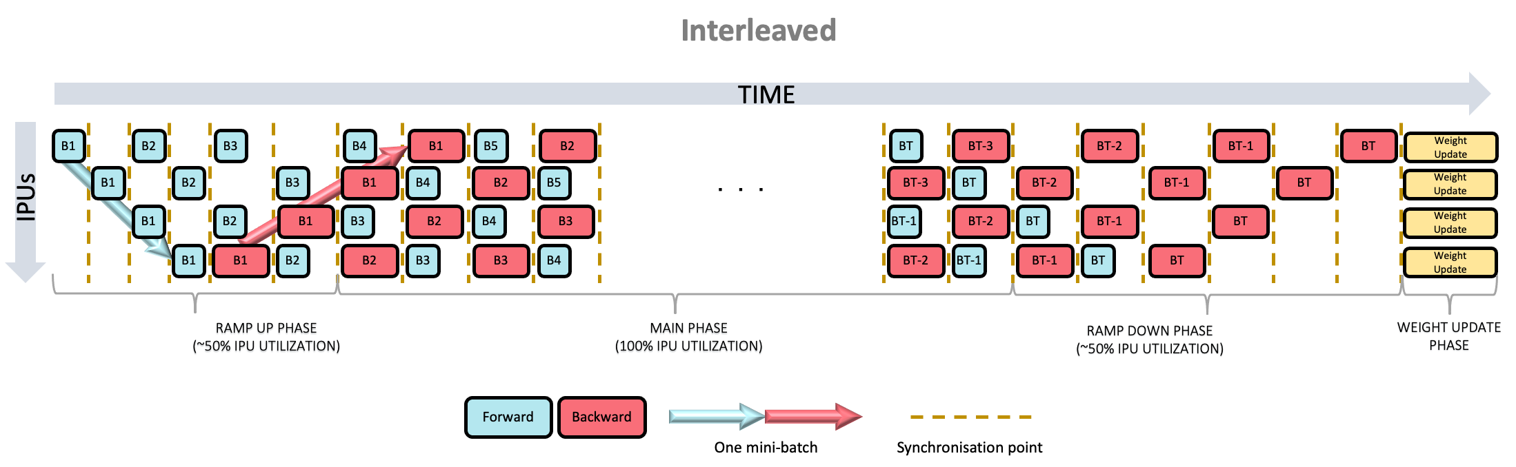
Fig. 5.2 Interleaved scheduling
5.4.3. Sequential scheduling
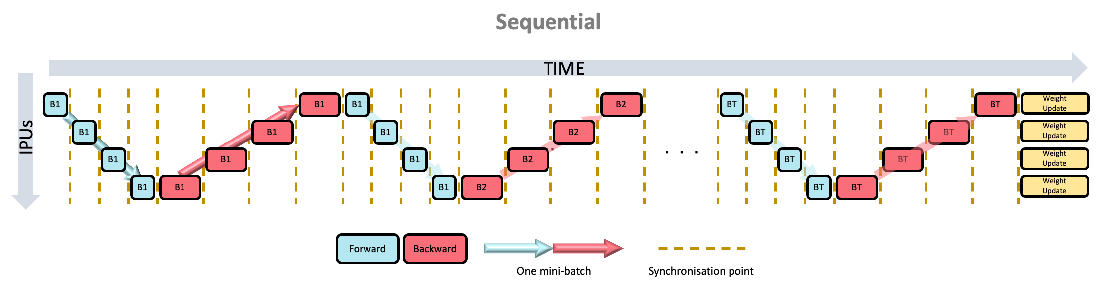
Fig. 5.3 Sequential scheduling
5.4.4. Pipeline stage inputs and outputs
The first pipeline stage needs to have inputs which are a combination of the tensors from the DataSet, and the tensors given as arguments to the pipeline operation. Any data which changes for every sample or minibatch of the input should be included in the DataSet, while data which can vary only on each run of the pipeline should be passed as arguments to the pipeline operation. Parameters like the learning rate would fit into this latter case.
Every subsequent pipeline stage must have its inputs as the outputs of the previous stage. Note that things like the learning rate must be threaded through each pipeline stage until they are used.
5.4.5. Applying an optimiser to the graph
The optimiser must be applied by creating it in a special optimiser function
and then returning a handle to it from that function. The function is passed
into the optimizer_function argument of the pipeline operation.
When a pipeline is running it will accumulate the gradients from each step of
the pipeline and only apply the updates to the graph parameters at the end of
each pipeline run, given by the gradient_accumulation_count parameter.
Consequently it is important for the system to have more knowledge of the
optimiser and so it must be given to the pipeline operator using this function.
5.4.6. Device mapping
By default the pipeline operation will map the pipeline stages onto IPUs in
order to minimise the inter-IPU communication lengths. If you need to
override this order, then you can use the device_mapping parameter.
5.4.7. Concurrent pipeline stages
When pipelining a model, it’s possible to have stages that have no data dependencies and don’t share weights. These stages can benefit from operating on the same mini-batch concurrently.
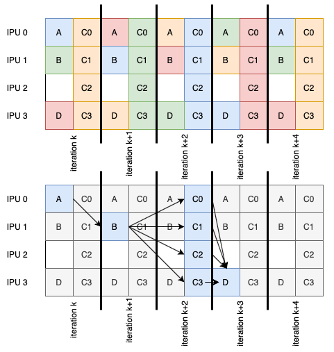
Fig. 5.4 An example pipeline with stages (lettered boxes) processing multiple mini-batches (colours of the stages). The flow of a single mini-batch is highlighted at the bottom.
These concurrent pipeline stages are defined by providing a list of stages. The corresponding element of the device-mapping should also be a list. The argument list to each concurrent stage must be the same, including any arguments coming from an infeed. The input to the next stage, or outfeed, is the concatenation of concurrent stage outputs.
def stage1a(args...):
  # ... do stuff on IPU 1
  return a0, a1, ...
def stage1b(args...):
  # ... do stuff on IPU 2
  return b0, b1, ...

# stage 2 arguments are a concatenation of the results of the previous
# concurrent stages.
def stage2(a0, a1, ..., b0, b1, ...):
  # ... do stuff on IPU 2

pipeline_op = pipelining_ops.pipeline(
  # Second element of the list is also a list of functions.
  computational_stages=[stage0, [stage1a, stage1b], stage2, stage3],
  # ...
  # Second element of the list is also a list of device IDs.
  device_mapping=[0, [1, 2], 2, 3])
Comparing this to a pipeline not using this feature where the activations are passed through stages, the pipeline is shorter. This means that fewer activations are stored over the whole execution of the pipeline and the expected latency is lower than the serialised pipeline.
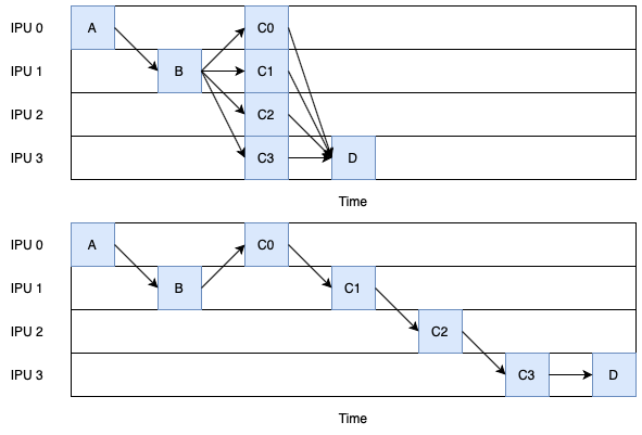
Fig. 5.5 Comparison of the same logical pipelines with concurrent stages (top) and without (bottom).
5.5. Gradient accumulation
Gradient accumulation is a technique for increasing the effective batch size by processing multiple batches of training examples before updating the model. The gradients from each batch are accumulated and these accumulated gradients are used to compute the weight update. When gradient accumulation is used, the effective batch size of the model is the number of mini-batches for which the gradients are accumulated multiplied by the mini-batch size.
Gradient accumulation is a useful optimisation technique for replicated graphs as it reduces the number of times the gradients are exchanged between replicas by a factor of the number of mini-batches. This is because the gradients only need to be exchanged between replicas when the weight update is computed. When gradient accumulation is used with replication, the effective batch size of the model is the number of mini-batches for which the gradients are accumulated multiplied by the mini-batch size multiplied by the replication factor.
The choice of gradient accumulation count impacts the time spent in the ramp-up and ramp-down stages of pipeline execution. As the gradient accumulation count increases, the proportion of cycles spent on the ramp-up/ramp-down phases decreases, with respect to the total number of cycles required to process the batch. As weight updates are performed after the ramp-down phase, a higher gradient accumulation count also results in a smaller proportion of cycles spent on weight updates.
There are multiple convenient ways to use gradient accumulation with minimal modifications to your model.
5.5.1. Optimizers
Gradient accumulation optimizers provide an easy way to add gradient accumulation to your model:
GradientAccumulationOptimizerV2is a general purpose optimizer which can be used to wrap any other TensorFlow optimizer. It supports optimizer state offloading (see the Optimizer state offloading section).GradientAccumulationOptimizeris an optimizer which can be used to wraptf.train.GradientDescentOptimizerandtf.train.MomentumOptimizeronly. Note that this optimizer does not support optimizer state offloading.
The cross-replica versions of these optimizers can be used with replicated
graphs, see
CrossReplicaGradientAccumulationOptimizerV2
and
CrossReplicaGradientAccumulationOptimizer.
Note
These optimizers need to be used inside of a training loop generated
by repeat().
5.5.2. Pipelining
All pipelined training graphs automatically apply gradient accumulation to the
model such that the weight update is only computed once all the mini-batches have
gone through the whole model pipeline, where the number of mini-batches is the
gradient_accumulation_count.
Note
Since the pipelined models always implement gradient accumulation, no gradient accumulation optimizer should be used in combination with pipelining.
You can also find a practical example of this in the Graphcore tutorials repository: Using pipelining for a simple model in TensorFlow.
5.5.3. Accumulation data type
When accumulating gradients over a large number of mini-batches, it can be
beneficial to perform the accumulation in a data type with higher precision
(and dynamic range) than that of the gradients. By default, the accumulation is
performed using the same data type as the corresponding variable, but this can
be overridden by passing gradient_accumulation_dtype (or just dtype to
the GradientAccumulationOptimizerV2).
This argument can be either of these three options:
None: Use an accumulator of the same type as the variable type.A
DType: Use this type for all the accumulators. For exampletf.float32.A callable that takes the variable and returns a
DType: Allows specifying the accumulator type on a per-variable basis. For example, passinglambda var: var.dtypewould have the same effect as passingNone.
Note that when accumulating the gradients using a different data type than that of the variable, an standard optimizer will not work since there will be a data type mismatch between the accumualated gradient and the variable when doing the weight update. You can use a custom optimizer to cast the final accumulated gradient to the data type of the variable before performing the weight update, for example like this with a Keras SGD optimizer:
class CastGradientsSGD(tf.keras.optimizers.SGD):
  def apply_gradients(self, grads_and_vars, name=None):
    cast_grads_and_vars = [(tf.cast(g, v.dtype), v)
                           for (g, v) in grads_and_vars]
    return super().apply_gradients(cast_grads_and_vars, name)
5.6. Optimizer state offloading
Some optimizers have an optimizer state which is only accessed and modified
during the weight update. For example the tf.MomentumOptimizer optimizer has
accumulator variables which are only accessed and modified during the weight
update.
This means that when gradient accumulation is used, whether through the use of
pipelining or the
GradientAccumulationOptimizerV2
optimizer, the optimizer state variables do not need to be stored in the device
memory during the forward and backward propagation of the model. These variables
are only required during the weight update and so they are streamed onto the
device during the weight update and then streamed back to remote memory after
they have been updated.
This feature is enabled by default for both pipelining and when
GradientAccumulationOptimizerV2
is used.
It can be disabled by setting the offload_weight_update_variables argument
of pipeline() or
GradientAccumulationOptimizerV2
to False.
This feature requires the machine to be configured with support for Poplar remote buffers and if the machine does not support it, it is disabled.
Offloading variables into remote memory can reduce maximum memory liveness, but it can also increase the computation time of the weight update as more time is spent communicating with the host.
5.7. Dataset benchmarking
In order to fully utilise the potential of the IPU, the tf.data.Dataset used
by the IPUInfeedQueue needs to be optimised so that the IPU is not constantly
waiting for more data to become available.
To benchmark your tf.data.Dataset, you can make use of the
ipu.dataset_benchmark tool.
See tensorflow.python.ipu.dataset_benchmark for details of the
functions that you can use to obtain the maximum throughput of your
tf.data.Dataset.
If the throughput of your tf.data.Dataset is the bottleneck, you can try to
optimise it using the information on the TensorFlow website:
5.7.1. Accessing the JSON data
The functions in ipu.dataset_benchmark return a JSON string which can
be loaded into a JSON object using the native JSON library, for example:
import tensorflow as tf
from tensorflow.python import ipu
import json

# Create your tf.data.Dataset
dataset = ...
benchmark_op = ipu.dataset_benchmark.dataset_benchmark(dataset, 10, 512)

with tf.Session() as sess:
    json_string = sess.run(benchmark_op)
    json_object = json.loads(json_string[0])
5.8. Half and mixed precision training
TensorFlow provides native support for using 16-bit floating point precision data types.
You can write your model or modify an existing model to perform some or all computations
using the native tf.float16 data type. To find out more about using half or mixed precision
data types for training models in TensorFlow, take a look at this tutorial from the Graphcore
tutorials repository:
TensorFlow 1 on the IPU: Training a model using half- and mixed-precision.