3. Pipelining

3.1. Overview

The pipeline approach is similar to sharding. The entire model is partitioned into multiple computing stages, and the output of a stage is the input of the next stage. These stages are executed in parallel on multiple IPUs. Compared to using sharding technology alone, the pipeline approach can maximise the use of all IPUs involved in parallel model processing, which improves processor efficiency as well as throughput and latency performance.

When discussing the use of pipelining, the following nomenclature applies:

• Mini-batch A set of data samples to be processed in a single forward pass.

• Batch A set of mini-batches to be processed by the pipeline. The total sample count of which is sometimes referred to as the effective batch size.

Within this context, it suffices to consider a pipeline to be fed mini-batches until a weight update is performed over the set of mini-batches (the batch).

Fig. 3.1 shows how to use pipelining for model parallelism (the dotted-line box indicates the point in the pipeline body where all IPUs are used to the maximum extent). The model consists of four layers and these are divided into four stages. Each stage is assigned to an IPU which computes a layer. When the first IPU receives a mini-batch of data B1 and the first stage is executed, the second IPU starts to execute the second stage and, at the same time, the first IPU receives the next mini-batch of data B2 and starts to execute the first stage, and so on. When the fourth mini-batch of data B4 is read, the parallelism of the four IPUs reaches 100%.

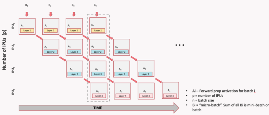
Fig. 3.1 Pipeline time sequence during model inference

The pipeline is relatively simple for inference, but more complicated for training based on backpropagation. For training, pipelining needs to adapt to include the forward pass, backpropagation and weight update.

Fig. 3.2 shows a single computational flow of forward pass and backpropagation, and then shows a complete pipeline with parallel overlapping mini-batches.

Each IPU performs not only the forward computation (Ai) of the corresponding layer, but also the gradient computation (AiGi). The dotted-line box shows the main body of the pipeline (it can be any depth, and larger depth can increase the size of the batch). Through the use of recomputation (see Section 3.5, Optimising the pipeline), the relevant IPU is used to the maximum extent to process forward activations, the previous activations are recomputed from the stored activation inputs, and the gradient updates are computed to save valuable on-chip memory.

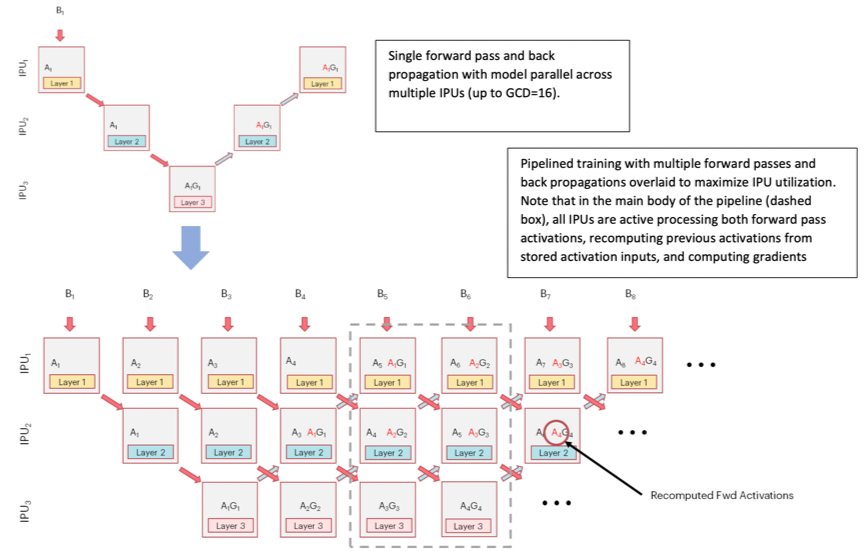
Fig. 3.2 Pipeline time sequence during model training

The GCD mentioned in the image stands for “graph compile domain”, and is a set of IPUs which the Poplar graph compiler will compile binaries for. With a GCD of size 16, for example, we can generate a model-parallel graph that executes on 16 IPUs.

3.2. Pipeline operation

There are three phases to the pipelined execution:

• Ramp up: this is the period in which the pipeline is being filled with mini-batches until every pipeline stage (including forward and backward passes) is performing computation. The maximum utilisation is 50%.

• Main execution: the time when all the pipeline stages are performing computation. This is the period when maximum utilisation is made of all the IPUs.

• Ramp down: the time when the pipeline is being drained until each pipeline stage is no longer performing any computation. The maximum utilisation is again 50%.

After ramp down, the weight updates are performed.

Note

Pipelining must not be combined with sharding.

3.3. Pipelining API

The pipelining API allows the you to describe what the forward, backward and weight update operations are. You define the forward stages. The backward stages and the weight updates are automatically generated. Check the pipelining interface in the TensorFlow API documentation.

3.3.1. Inputs and outputs

All tensors which are used in the pipeline that are not TensorFlow variables need to be explicitly passed as inputs to the pipeline. If the input passed in does not change value – for example, hyper-parameters – add them to the inputs argument.

If the input does change value with every execution of a pipeline stage – for example, mini-batches of data – then create an IPUInfeedQueue and pass it to the infeed_queue argument. The inputs list and the infeed_queue are passed as inputs to the first pipeline stage.

After the initial pipeline stage, all the outputs of a pipeline stage N are passed as inputs to the pipeline stage N+1. If an output of a stage N is used by a stage N+M where M > 1, then that output will be passed through the stages in between.

If the last computational stage has any outputs – for example, loss or the prediction – then you will need to create an IPUOutfeedQueue and pass it to the outfeed_queue argument. All the outputs from the final computational stage are passed to the outfeed automatically.

3.3.2. Device mapping

By default, the pipeline stages will be assigned to IPU devices in an order which should maximise the utilisation of IPU-Links between consecutive pipeline stages.

If your model is not sequential you might want to change the assignment, depending on the communication pattern in your model.

Any TensorFlow variables can only be used by pipeline stages which are on the same IPU. You can use the device mapping API to assign pipeline stages which use the same variable to be on the same IPU.

3.3.3. Pipeline scheduling

You can choose the method used for scheduling the operations in the pipeline. The scheduling methods have different trade-offs in terms of memory use, balancing computation between pipeline stages (and therefore the IPUs), and optimisations that can be applied. They will also have different pipeline depths and therefore different ramp-up and ramp-down times. The differences are most significant when training and you may need to experiment to find which method works best for your model.

There are three pipeline schedules:

• grouped

• interleaved

• sequential

In the grouped schedule (Fig. 3.3) the forward and backward stages are grouped together on each IPU. All IPUs alternate between executing a forward pass and then a backward pass.

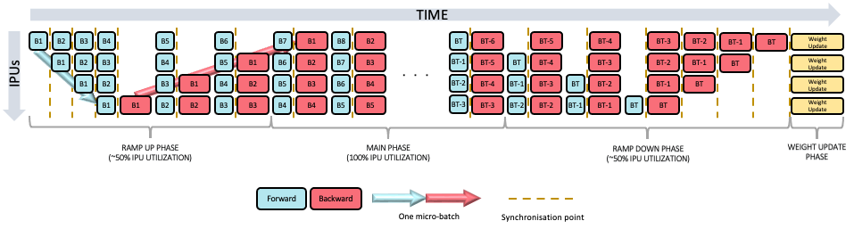
Fig. 3.3 Grouped schedule

In the interleaved schedule (Fig. 3.4) each pipeline stage executes a combination of forward and backward passes.

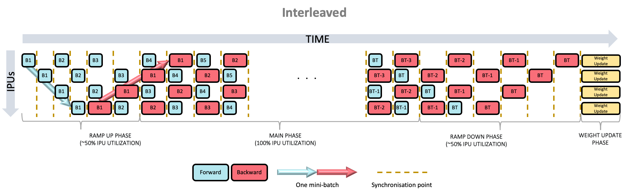
Fig. 3.4 Interleaved schedule

Finally, there is the sequential schedule (Fig. 3.5). This is the same as sharding a model: only one mini-batch is ever “in-flight”. This may be useful when you cannot have a big mini-batch size but want to make use of other pipeline features, such as recomputation.

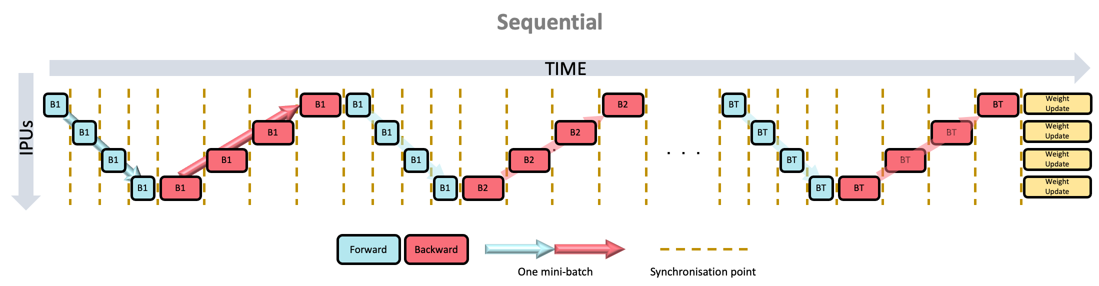
Fig. 3.5 Sequential schedule

The grouped and interleaved schedules have different advantages and disadvantages for:

• memory use

• execution time

• ramp up and ramp down time

• inter-IPU optimisations

Memory use

For a pipeline with N stages:

• The grouped schedule executes 2N mini-batches at any given time.

• The interleaved schedule executes N mini-batches at any given time.

• This means that the interleaved schedule requires less memory for the storing the data to be transferred between forward and backward passes.

Execution time

• The grouped schedule executes all the forward stages together and all the backward stages together.

• The interleaved schedule executes the forward stages and backward stages interleaved.

• Due to the synchronisation required between stages, and the fact that the forward stages tend to use fewer cycles than the backward stages, the grouped schedule is likely to be faster.

Ramp-up and ramp-down time

For a pipeline with N stages:

• The grouped schedule executes 2N mini-batches in total to perform the ramp up and ramp down.

• The interleaved schedule executes N mini-batches in total to perform the ramp up and ramp down.

Inter-IPU optimisations

• Some inter-IPU optimisations are not possible with the interleaved schedule. For example, an optimisation which converts variables which are passed through multiple pipeline stages into FIFOs.

3.3.4. Keras API in TensorFlow 2

TensorFlow 2 for the IPU includes the Keras Model and Sequential classes with IPU specific arguments passed into separate configuration methods. For more details check the TensorFlow API documentation.

3.4. Code examples

3.4.1. Inference code examples

The following code shows an example usage of the pipeline API in TensorFlow 1.

from tensorflow.python.ipu import config
from tensorflow.python.ipu import ipu_compiler
from tensorflow.python.ipu import ipu_infeed_queue
from tensorflow.python.ipu import ipu_outfeed_queue
from tensorflow.python.ipu.ops import pipelining_ops
from tensorflow.python.data.ops.dataset_ops import Dataset
from tensorflow.python.ipu import scopes
from tensorflow.python.ipu import utils
from tensorflow.python.framework import ops
from tensorflow.python.ops import variables
from tensorflow.keras import layers
import numpy as np
import tensorflow.compat.v1 as tf

tf.disable_v2_behavior()

# default data_format is 'channels_last'
dataset = Dataset.from_tensor_slices(np.random.uniform(size=(2, 128, 128, 3)).astype(np.float32))
dataset = dataset.batch(batch_size=2, drop_remainder=True)
dataset = dataset.cache()
dataset = dataset.repeat()
dataset = dataset.prefetch(tf.data.experimental.AUTOTUNE)

# Create the data queues from/to IPU.
infeed_queue = ipu_infeed_queue.IPUInfeedQueue(dataset)
outfeed_queue = ipu_outfeed_queue.IPUOutfeedQueue()

# Create a pipelined model which is split accross two stages.
def stage1(x):
    x = layers.Conv2D(128, 1)(x)
    return x

def stage2(x):
    x = layers.Conv2D(128, 1)(x)
    return x

def my_net():
    pipeline_op = pipelining_ops.pipeline(
                        computational_stages=[stage1, stage2],
                        gradient_accumulation_count=16,
                        repeat_count=2,
                        inputs=[],
                        infeed_queue=infeed_queue,
                        outfeed_queue=outfeed_queue,
                        name="Pipeline")
    return pipeline_op

with ops.device("/device:IPU:0"):
    r = ipu_compiler.compile(my_net, inputs=[])

dequeue_op = outfeed_queue.dequeue()

cfg = config.IPUConfig()
cfg.auto_select_ipus = 2
cfg.configure_ipu_system()
utils.move_variable_initialization_to_cpu()

with tf.Session() as sess:
    sess.run(variables.global_variables_initializer())
    sess.run(infeed_queue.initializer)
    sess.run(r)
    output = sess.run(dequeue_op)

The code first creates a dataset with infeed_queue and outfeed_queue which are for data input and output. The functions stage1() and stage2() define two computation stages. The most important definitions are in my_net() which defines the entire behaviour of the pipeline. Among them:

• computational_stages indicates that the stage list contains stage1 and stage2

• gradient_accumulation_count=16 means that each pipeline stage is executed 16 times before the weights are updated

• repeat_count=2 means that the whole pipeline is executed twice

The program selects two IPUs to perform this task using auto_select_ipus, and each stage is automatically assigned to a single IPU.

The following example uses the Keras API in TensorFlow 2 to define a model equivalent to the one in the example above.

from tensorflow.python.data.ops.dataset_ops import Dataset
from tensorflow.python.ipu import utils
from tensorflow.keras import layers
from tensorflow.python.ipu import config
from tensorflow.python.ipu import ipu_strategy
import numpy as np
import tensorflow as tf
from tensorflow.python import ipu

# default data_format is 'channels_last'
dataset = Dataset.from_tensor_slices(np.random.uniform(size=(2, 128, 128, 3)).astype(np.float32))
dataset = dataset.batch(batch_size=2, drop_remainder=True)
dataset = dataset.cache()
dataset = dataset.repeat()
dataset = dataset.prefetch(tf.data.experimental.AUTOTUNE)

# Create a pipelined model which is split accross two stages.
def my_model():
    input_layer = layers.Input(shape=(128, 128, 3), dtype=tf.float32, batch_size=2)

    with ipu.keras.PipelineStage(0):
        x = layers.Conv2D(128, 1)(input_layer)

    with ipu.keras.PipelineStage(1):
        x = layers.Conv2D(128, 1)(x)

    return tf.keras.Model(input_layer, x)

cfg = config.IPUConfig()
cfg.auto_select_ipus = 2
cfg.configure_ipu_system()
utils.move_variable_initialization_to_cpu()

# Define the model under an IPU strategy scope
strategy = ipu_strategy.IPUStrategy()
with strategy.scope():
    model = my_model()
    model.set_pipelining_options(gradient_accumulation_steps_per_replica=16)

    model.compile(steps_per_execution=10)
    model.predict(dataset, steps=2)

When defining a model for use with tf.keras.Model, the computational stages are defined by the layers under the PipelineStage scopes. In TensorFlow 2, to ensure that the model will be compiled for the IPUs, we enclose it in an IPUstrategy scope.

Note the use of set_pipelining_options method, which is used to set the gradient_accumulation_steps_per_replica parameter (equivalent to gradient_accumulation_count in the TensorFlow 1 example above). After this, the program calls compile() and predict() methods to run inference on the model.

The steps_per_execution argument helps reduce Python overhead and maximize the performance of your model. For more information, check the instructions on how to use this argument.

The following is the same model defined using tf.keras.Sequential:

from tensorflow.python.data.ops.dataset_ops import Dataset
from tensorflow.python.ipu import utils
from tensorflow.keras import layers
from tensorflow.python.ipu import config
from tensorflow.python.ipu import ipu_strategy
import numpy as np
import tensorflow as tf

# default data_format is 'channels_last'
dataset = Dataset.from_tensor_slices(np.random.uniform(size=(2, 128, 128, 3)).astype(np.float32))
dataset = dataset.batch(batch_size=2, drop_remainder=True)
dataset = dataset.cache()
dataset = dataset.repeat()
dataset = dataset.prefetch(tf.data.experimental.AUTOTUNE)

# Create a pipelined model which is split accross two stages.
def my_model():
    return tf.keras.Sequential([layers.Conv2D(128, 1),
                                layers.Conv2D(128, 1)])

cfg = config.IPUConfig()
cfg.auto_select_ipus = 2
cfg.configure_ipu_system()
utils.move_variable_initialization_to_cpu()

# Define the model under an IPU strategy scope
strategy = ipu_strategy.IPUStrategy()
with strategy.scope():
    model = my_model()

    model.set_pipeline_stage_assignment([0, 1])
    model.set_pipelining_options(gradient_accumulation_steps_per_replica=16)

    model.compile(steps_per_execution=10)
    model.predict(dataset, steps=2)

The only differences from tf.keras.Model is how the model is defined, as well as how the pipeline stages are assigned - using model.set_pipeline_stage_assignment() instead of keras.PipelineStage().

It is possible to use model.set_pipeline_stage_assignment() with tf.keras.Model or any functional model, which is useful for pipelining already existing models:

from tensorflow.python.data.ops.dataset_ops import Dataset
from tensorflow.python.ipu import utils
from tensorflow.keras import layers
from tensorflow.python.ipu import config
from tensorflow.python.ipu import ipu_strategy
import numpy as np
import tensorflow as tf

# default data_format is 'channels_last'
dataset = Dataset.from_tensor_slices(np.random.uniform(size=(2, 128, 128, 3)).astype(np.float32))
dataset = dataset.batch(batch_size=2, drop_remainder=True)
dataset = dataset.cache()
dataset = dataset.repeat()
dataset = dataset.prefetch(tf.data.experimental.AUTOTUNE)

# Create a pipelined model which is split across two stages.
def my_model():
    input_layer = layers.Input(shape=(128, 128, 3), dtype=tf.float32, batch_size=2)

    x = layers.Conv2D(128, 1)(input_layer)

    x = layers.Conv2D(128, 1, name='split')(x)

    x = layers.Conv2D(128, 1)(x)

    x = layers.Conv2D(128, 1)(x)

    return tf.keras.Model(input_layer, x)

cfg = config.IPUConfig()
cfg.auto_select_ipus = 2
cfg.configure_ipu_system()
utils.move_variable_initialization_to_cpu()

# Define the model under an IPU strategy scope
strategy = ipu_strategy.IPUStrategy()
with strategy.scope():
    model = my_model()

    # Get the individual assignments - note that they are returned in post-order.
    assignments = model.get_pipeline_stage_assignment()

    # Iterate over them and set their pipeline stages.
    stage_id = 0
    for assignment in assignments:
        assignment.pipeline_stage = stage_id
        if assignment.layer.name.startswith("split"):
            stage_id = 1

    # Set the assignments to the model.
    model.set_pipeline_stage_assignment(assignments)
    model.set_pipelining_options(gradient_accumulation_steps_per_replica=16)

    model.compile(steps_per_execution=10)
    model.predict(dataset, steps=2)

This includes two extra steps:

• Getting the individual assignments of the layers using model.get_pipeline_stage_assignment()

• Setting the pipeline stages.

You can name your layers using the name parameter and call assignment.layer.name.startswith("NAME") inside the pipeline stage assignment to move to the next pipeline stage.

In the example above, the first two layers are part of the first pipeline stage and the last two are part of the second pipeline stage.

3.4.2. Training code examples

This example creates a pipeline of four stages with gradient accumulation count of 8 and a repeat count of 2. Four IPUs are selected for computation.

The selection order is ZIGZAG, and recomputation is enabled. The loss function is cross-entropy, and the optimiser is tf.train.GradientDescentOptimizer().

The source code is shown below (TensorFlow 1):

from tensorflow.python.ipu import config
from tensorflow.python.ipu import ipu_compiler
from tensorflow.python.ipu import ipu_infeed_queue
from tensorflow.python.ipu import ipu_outfeed_queue
from tensorflow.python.ipu.ops import pipelining_ops
from tensorflow.python.ops import variable_scope
from tensorflow.python.data.ops.dataset_ops import Dataset
from tensorflow.python.ipu import utils
from tensorflow.python.framework import ops
from tensorflow.python.ops import variables
from tensorflow.keras import layers
import numpy as np
import tensorflow.compat.v1 as tf

tf.disable_v2_behavior()

# default data_format is 'channels_last'
dataset = Dataset.from_tensor_slices(
    (tf.random.uniform([2, 128, 128, 3], dtype=tf.float32),
    tf.random.uniform([2], maxval=10, dtype=tf.int32))
    )
dataset = dataset.batch(batch_size=2, drop_remainder=True)
dataset = dataset.shuffle(1000)
dataset = dataset.cache()
dataset = dataset.repeat()
dataset = dataset.prefetch(tf.data.experimental.AUTOTUNE)

# Create the data queues from/to IPU.
infeed_queue = ipu_infeed_queue.IPUInfeedQueue(dataset)
outfeed_queue = ipu_outfeed_queue.IPUOutfeedQueue()

# Create a pipelined model which is split accross four stages.
def stage1(x, labels):
    with variable_scope.variable_scope("stage1", use_resource=True):
        with variable_scope.variable_scope("conv", use_resource=True):
            x = layers.Conv2D(3, 1)(x)
            return x, labels

def stage2(x, labels):
    with variable_scope.variable_scope("stage2", use_resource=True):
        with variable_scope.variable_scope("conv", use_resource=True):
            x = layers.Conv2D(3, 1)(x)
            return x, labels

def stage3(x, labels):
    with variable_scope.variable_scope("stage3", use_resource=True):
        with variable_scope.variable_scope("conv", use_resource=True):
            x = layers.Conv2D(3, 1)(x)
            return x, labels

def stage4(x, labels):
    with variable_scope.variable_scope("stage3", use_resource=True):
        with variable_scope.variable_scope("flatten", use_resource=True):
            x = layers.Flatten()(x)
        with variable_scope.variable_scope("dense", use_resource=True):
            logits = layers.Dense(10)(x)
        with variable_scope.variable_scope("entropy", use_resource=True):
            cross_entropy = tf.nn.sparse_softmax_cross_entropy_with_logits(
                labels=labels, logits=logits)
        with variable_scope.variable_scope("loss", use_resource=True):
            loss = tf.reduce_mean(cross_entropy)
        return loss

def optimizer_function(loss):
    optimizer = tf.train.GradientDescentOptimizer(0.01)
    return pipelining_ops.OptimizerFunctionOutput(optimizer, loss)

def my_net():
    pipeline_op = pipelining_ops.pipeline(
                        computational_stages=[stage1, stage2, stage3, stage4],
                        gradient_accumulation_count=8,
                        repeat_count=2,
                        inputs=[],
                        infeed_queue=infeed_queue,
                        outfeed_queue=outfeed_queue,
                        optimizer_function=optimizer_function,
                        name="Pipeline")
    return pipeline_op

with ops.device("/device:IPU:0"):
    r = ipu_compiler.compile(my_net, inputs=[])

dequeue_op = outfeed_queue.dequeue()

cfg = config.IPUConfig()
cfg.allow_recompute = True
cfg.selection_order = config.SelectionOrder.ZIGZAG
cfg.auto_select_ipus = 4
cfg.configure_ipu_system()
utils.move_variable_initialization_to_cpu()

with tf.Session() as sess:
    sess.run(variables.global_variables_initializer())
    sess.run(infeed_queue.initializer)
    sess.run(r)
    losses = sess.run(dequeue_op)

Here, tf.train.GradientDescentOptimizer() automatically adds a stage to the pipeline for gradient computation, and a stage (gradientDescent) for weight update. Note that gradient_accumulation_count=8 means that gradientDescent is computed once every eight mini-batches of data. And repeat_count=2 means that the pipeline computes twice the gradientDescent; that is, the weight parameters are updated twice.

You can profile the program by running it with the following environment variable POPLAR_ENGINE_OPTIONS='{"autoReport.all":"true", "autoReport.directory":"/destination/path/"}', and then open the generated report with PopVision Graph Analyser to get the execution information as shown in Fig. 3.6. Check also Section 4, PopVision™ Graph Analyser tool for further information.

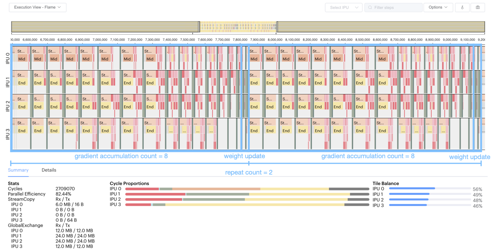
Fig. 3.6 Training pipeline profile

We can see from this figure that:

• The pipeline is repeated twice.

• Each repetition of the pipeline computes eight mini-batches of data.

• Each mini-batch of data goes through the phases of forward pass and gradient computation (with optional recomputation).

• Four stages are executed in parallel on four IPUs.

• After eight gradient computations, a gradient descent will be executed, that is, the weight will be updated once for the batch.

Below we show equivalent programs that use pipelining for training, using TensorFlow 2 and the tf.keras.Model and tf.keras.Sequential classes.

from tensorflow.python.data.ops.dataset_ops import Dataset
from tensorflow.python.ipu import utils
from tensorflow.keras import layers
from tensorflow.keras import optimizers
from tensorflow.python.ipu import config
from tensorflow.python.ipu import ipu_strategy
import numpy as np
import tensorflow as tf
from tensorflow.python import ipu

# default data_format is 'channels_last'
dataset = Dataset.from_tensor_slices(
    (tf.random.uniform([2, 128, 128, 3], dtype=tf.float32),
    tf.random.uniform([2], maxval=10, dtype=tf.int32))
    )
dataset = dataset.batch(batch_size=2, drop_remainder=True)
dataset = dataset.shuffle(1000)
dataset = dataset.cache()
dataset = dataset.repeat()
dataset = dataset.prefetch(tf.data.experimental.AUTOTUNE)

# Create a pipelined model which is split accross four stages.
def my_model():
    input_layer = layers.Input(shape=(128, 128, 3), dtype=tf.float32, batch_size=2)

    with ipu.keras.PipelineStage(0):
        x = layers.Conv2D(3, 1)(input_layer)

    with ipu.keras.PipelineStage(1):
        x = layers.Conv2D(3, 1)(x)

    with ipu.keras.PipelineStage(2):
        x = layers.Conv2D(3, 1)(x)

    with ipu.keras.PipelineStage(3):
        x = layers.Flatten()(x)
        logits = layers.Dense(10)(x)

    return tf.keras.Model(input_layer, logits)

cfg = config.IPUConfig()
cfg.allow_recompute = True
cfg.selection_order = config.SelectionOrder.ZIGZAG
cfg.auto_select_ipus = 4
cfg.configure_ipu_system()
utils.move_variable_initialization_to_cpu()

# Define the model under an IPU strategy scope
strategy = ipu_strategy.IPUStrategy()
with strategy.scope():
    model = my_model()
    model.set_pipelining_options(gradient_accumulation_steps_per_replica=8)

    model.compile(steps_per_execution=128,
                  loss='sparse_categorical_crossentropy',
                  optimizer=optimizers.SGD(0.01))

    model.fit(dataset, steps_per_epoch=128)

And finally the tf.keras.Sequential version, which differs from the above only in the definition of the model, as in the inference code examples.

from tensorflow.python.data.ops.dataset_ops import Dataset
from tensorflow.python.ipu import utils
from tensorflow.keras import layers
from tensorflow.keras import optimizers
from tensorflow.python.ipu import config
from tensorflow.python.ipu import keras
from tensorflow.python.ipu import ipu_strategy
import numpy as np
import tensorflow as tf

# default data_format is 'channels_last'
dataset = Dataset.from_tensor_slices(
    (tf.random.uniform([2, 128, 128, 3], dtype=tf.float32),
    tf.random.uniform([2], maxval=10, dtype=tf.int32))
    )
dataset = dataset.batch(batch_size=2, drop_remainder=True)
dataset = dataset.shuffle(1000)
dataset = dataset.cache()
dataset = dataset.repeat()
dataset = dataset.prefetch(tf.data.experimental.AUTOTUNE)

# Create a pipelined model which is split accross four stages.
def my_model():
    return tf.keras.Sequential([layers.Conv2D(3, 1),
                                layers.Conv2D(3, 1),
                                layers.Conv2D(3, 1),
                                layers.Flatten(),
                                layers.Dense(10)])

cfg = config.IPUConfig()
cfg.allow_recompute = True
cfg.selection_order = config.SelectionOrder.ZIGZAG
cfg.auto_select_ipus = 4
cfg.configure_ipu_system()
utils.move_variable_initialization_to_cpu()

# Define the model under an IPU strategy scope
strategy = ipu_strategy.IPUStrategy()
with strategy.scope():
    model = my_model()

    model.set_pipelining_options(gradient_accumulation_steps_per_replica=8)
    model.set_pipeline_stage_assignment([0, 1, 2, 3, 3])

    model.compile(steps_per_execution=128,
                loss='sparse_categorical_crossentropy',
                optimizer=optimizers.SGD(0.01))

    model.fit(dataset, steps_per_epoch=128)

3.5. Optimising the pipeline

3.5.1. Recomputation

The Poplar SDK makes more efficient use of the valuable In-Processor-Memory by saving selected activation inputs, optimising on memory savings vs TFLOP expenditure with recomputation. The two figures below demonstrate this, showing how the subset of activation inputs that are saved can be used to recompute all the necessary activation history for the backward pass calculation of the weight updates, thus saving on memory usage. To enable recomputation, use the allow_recompute attribute of an instance of the IPUConfig class when configuring the device.

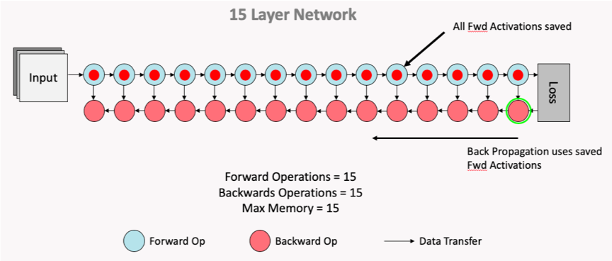
Fig. 3.7 Normal computation flow

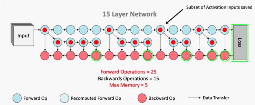
Fig. 3.8 Computation flow after recomputation enabled

3.5.2. Variable offloading

When using pipelining to train a model, it is possible to offload certain variables into Streaming Memory. This feature can allow savings of In-Processor-Memory memory, at the cost of time spent communicating with the host when the offloaded variables are needed on the device. The API supports offloading of the weight update variables and activations.

The weight update variables are any tf.Variable only accessed and modified during the weight update of the pipeline. An example is the accumulator variable of the tf.MomentumOptimizer. This means that these variables do not need to be stored in the device memory during the forward and backward propagation of the model, so when offload_weight_update_variables is enabled they are streamed onto the device during the weight update and then streamed back to Streaming Memory after they have been updated.

When offload_activations is enabled, all the activations for the mini-batches which are not being executed by the pipeline stages at any given time are stored in the Streaming Memory. So in an analogous way as described above, when an activation is needed for computation it is streamed onto the device, and then streamed back to the Streaming Memory after it has been used.

For more information on variable offloading, see the TensorFlow API documentation: Optimizer state offloading.

3.5.3. Device selection order

Use the API to make sure the pipeline stage mapping to devices utilises the IPU-Links as much as possible.

3.5.4. Data parallelism

Pipelining supports replicated graphs. When using the pipeline operator, use the tensorflow.python.ipu.optimizers.CrossReplicaOptimizer in the optimiser function. When using the IPU Keras PipelineModel and PipelineSequential from within an IPUStrategy, replication is handled automatically whenever the model is placed on a multi-IPU device and the CrossReplicaOptimizer must not be used.

If the model you are working on is defined as using a mini-batch size B and the gradient accumulation count is G and the replication factor is R, this results in an effective batch size of B x G x R.

Note that the all-reduce collectives for the gradients are only performed during the weight update.

3.5.5. Increase the gradient accumulation count

The bigger the gradient accumulation count:

• The smaller the proportion of time spent during a weight update.

• The smaller the proportion of time spent during ramp up and ramp down.

An increase in gradient accumulation count yields these reductions by performing the forward and backward passes on a greater number of mini-batches prior to the updating of weights and/or parameters, resulting in a greater effective batch size. The computed gradients for each mini-batch are aggregated such that the weight update is performed with the larger, aggregated batch.

In Fig. 3.9, the processing of four mini-batches is shown without gradient accumulation. It can be seen that following the forward and backward passes of each mini-batch is a weight update stage.

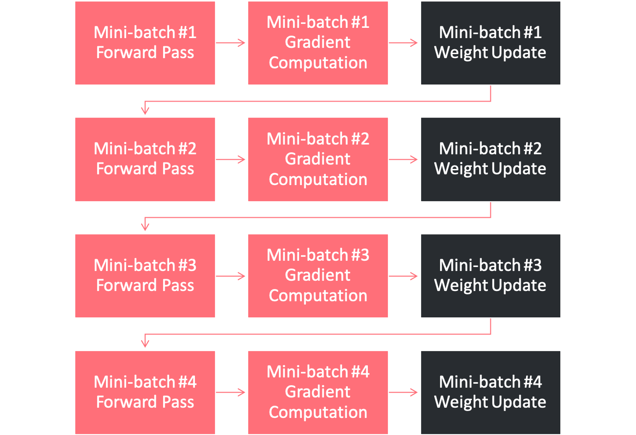
Fig. 3.9 Not using gradient accumulation

However, when processing the four-mini batches of Fig. 3.9 with a gradient accumulation count of four, it can be seen in Fig. 3.10 that only a single weight update stage is performed. This is due to the aggregation of the gradients computed in the backward pass for each mini-batch.

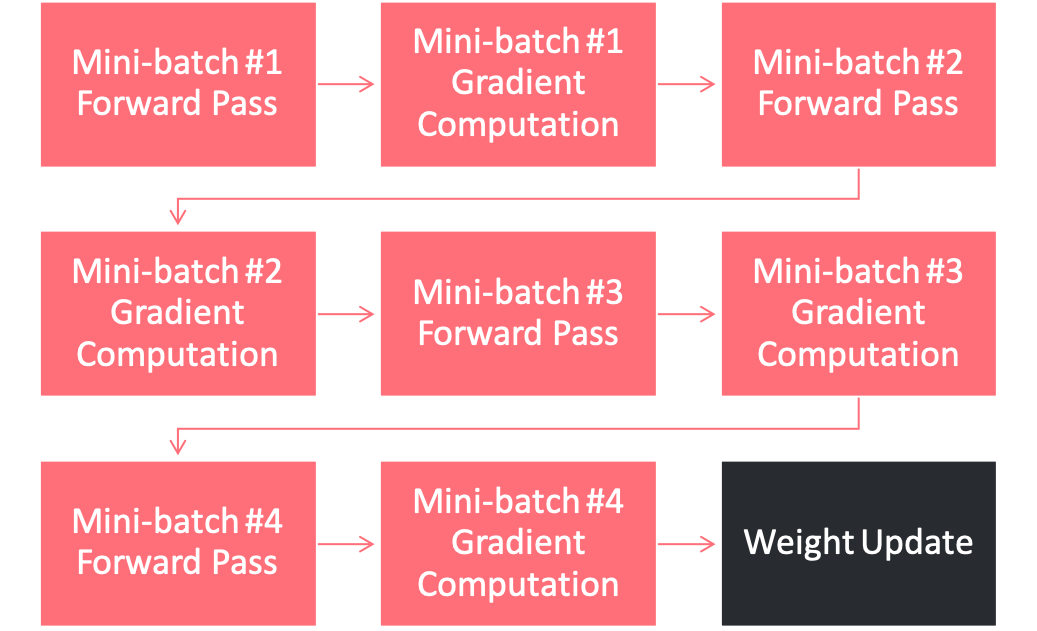
Fig. 3.10 Using a gradient accumulation count of 4

As weight updates are performed following the ramp down phase of pipeline execution, the use of a higher gradient accumulation count will also reduce the number of ramp up/ramp down cycles between batches as the effective batch size will be larger, as previously outlined. As ramp up and ramp down fill and clear the pipeline, reducing occurences of ramp up and ramp down maximises time spent on compute. A lower gradient accumulation count will incur more ramp up/ramp down cycles, causing more time to be spent filling and clearing the pipeline.

3.5.6. Profiling

When your model is executing correctly, you can try moving layers around, or if the model doesn’t fit in one or more IPUs you can try changing the available memory proportion for temporary memory usage (for more information, see the technical note on this option).

• Move layers towards the final computation stage to reduce the amount of recomputation

• Adjust availableMemoryProportion. For example:

# Set "availableMemoryProportion" flag to "0.5"
cfg = ipu.config.IPUConfig()
cfg.convolutions.poplar_options["availableMemoryProportion"] = "0.5"
cfg.matmuls.poplar_options["availableMemoryProportion"] = "0.5"
cfg.configure_ipu_system()

• More fine-grained control of the available memory proportion with the following options:

  • forward_propagation_stages_poplar_options: If provided, a list of length equal to the number of computational stages. Each element is a PipelineStageOptions object which allows for fine grain control of the Poplar options for a given forward propagation computational stage.

  • backward_propagation_stages_poplar_options: If provided, a list of length equal to the number of computational stages. Each element is a PipelineStageOptions object which allows for fine grained control of the Poplar options for a given backward propagation computational stage.

  • weight_update_poplar_options: If provided, a PipelineStageOptions object which allows for fine grained control of the Poplar options for the weight update stage.

  These can be useful in certain situations, for example if one stage is almost out of memory then the available memory proportion can be lowered there but not for the rest of the model.

• Make sure that the tf.Dataset passed to the pipeline is not the bottleneck. See the Dataset benchmarking section in Targeting the IPU from TensorFlow for more information.

• Experiment with Poplar engine options. For example:

POPLAR_ENGINE_OPTIONS='{"opt.enableSwSyncs": ”true"}'