1. Introduction
BERT (Bidirectional Encoder Representations from Transformers) is a transformer-based language representation model created by Google. Unlike previous transformer models, such as the Generative Pre-trained Transformer (GPT), it was designed to take advantage of the left and right context of each unlabelled training example in all transformer layers and effectively retrieve its bidirectional representations.
When BERT was first released in late 2018, around 10% of English search queries in Google employed BERT. During the past two years, BERT has been used in almost 100% of cases in English. As well as search engines, BERT has also been applied to other domains such as question answering, content-based recommendation, video understanding, protein feature extraction and many others.
BERT’s ability to use a vast unlabelled dataset in the pre-training phase, and to achieve state-of-the-art accuracy in the fine-tuning phase with a small amount of labelled data, makes large BERT-like transformer-based language models very attractive. As a result, the demand for training and fine-tuning these large neural-network language models is growing dramatically.
In order to meet such demands and pre-train billions of samples in days or even hours, the development of new AI hardware and highly-efficient scalable systems are imperative to support peta- or exaFLOPS computation, with high-speed interconnect and intelligent memory management. Graphcore’s scalable IPU‑POD systems are the ideal choice to meet these requirements.
As described in Devlin et al. 2018, we can see that it is not just large-scale tasks, such as language modelling, but also very small-scale downstream tasks that can benefit from these approaches.
For example, the Microsoft Research Paraphrase Corpus (MRPC) has only 3600 training samples, but the accuracy is increased from 84.4 to 86.6% by increasing the model size from BERT-Base to BERT-Large. BERT variants retain the lead over MRPC and many similar benchmarks. As ML researchers and engineers seek to further improve the task performance of these models, total model sizes continue to grow. This can be seen both within the BERT model variants and other more recent models, the largest of which now have over 100 billion parameters.
2. Pre-training BERT on the IPU-POD
It’s not just advances in modelling that make this possible, the development of new AI hardware and new AI systems is also important to enable us to train these models within reasonable times. Graphcore’s IPU‑POD addresses this performance challenge and greatly increases productivity for researchers and engineers.
In order to efficiently run BERT on the IPU‑POD, we load the entire model’s parameters on to the IPUs. To do this, the BERT model is split, or “sharded”, across four IPUs and executed as a pipeline during the training process.
The pipeline in Fig. 2.1 shows how we partition BERT-Large, where IPU 0 contains the embedding layer and projection/loss layers along with three encoder layers. The remaining 21 layers are evenly distributed over the other three IPUs. Since the embedding and projection layers share parameters, we place the projection, masked language model (MLM) and next sentence prediction (NSP) layers back on IPU 0.
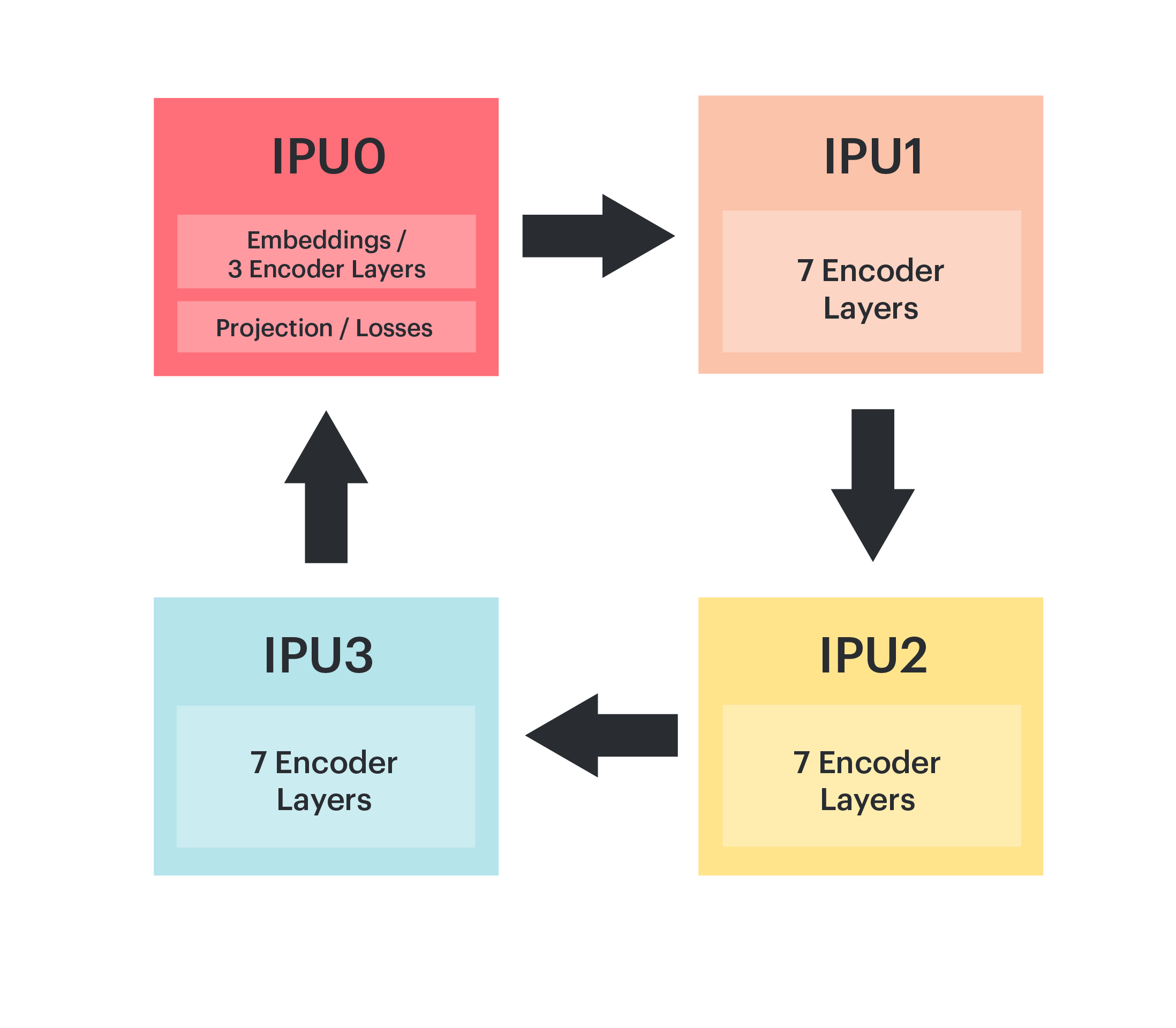
Fig. 2.1 Model parallelism of BERT-Large on an IPU‑POD4
In order to reduce the memory footprint on chip, recomputation is used (see Chen et al. 2016). This avoids having to store intermediate layer activations for use when calculating the backward passes. Recomputation is a strategy which can be used generally when training models; however, it is particularly useful when pipelining since we have multiple batches “in-flight” through the pipeline at any time and so the size of stored activations, without using recomputation, can be significant.
The optimizer state for the pre-training system is stored in Streaming Memory and loaded on demand during the optimizer step.
See the Graphcore examples for implementations of BERT for the IPU in TensorFlow, PyTorch and PopART.
Our TensorFlow 1 implementation shares model code with the original Google BERT implementation, with customization and extension to leverage Graphcore’s TensorFlow pipelining APIs.
Our PyTorch implementation is based on model descriptions and utilities from the Hugging Face transformers library. We use the Graphcore PopTorch library to target the IPU, including pipelined execution, recomputation and multi-replica/data parallelism.
We also provide a BERT implementation using the Poplar Advanced Runtime (PopART). PopART enables you to import or create models from an ONNX model description, and supports both training and inference. PopART supports optimizer, gradient and parameter partitioning as described in Rajbhandari et al. 2019. We collectively describe these as replicated tensor sharding (RTS). For our replicated pipeline model-parallel BERT system in PopART we use optimizer and gradient partitioning.
3. Scaling BERT to the IPU-POD
Unsupervised pre-training enables BERT to take advantage of the billions of training samples in Wikipedia, BookCorpus and other sources. Even with the IPU‑POD4, multiple passes over these large datasets take a significant amount of time. To further improve training time and researchers’ productivity we can use data-parallel model training to scale the pre-training process to IPU‑POD16, IPU‑POD64 and beyond.
Data-parallel training involves breaking the training dataset up into multiple parts, which are each consumed by a model replica. At each optimization step, the gradients are mean-reduced across all replicas to enable the weight update and model state to be the same across all replica.
3.1. Collective gradient reduction
The gradient reduction uses the Graphcore Communication Library (GCL) which implements a range of communication primitives, including a highly efficient ring-based collective all-reduce. Gradients are averaged across all replicas as illustrated in Fig. 3.1, and weight updates are applied once all multi-replica gradients are fully reduced.
Data-parallel gradient reduction can be added automatically using optimizer wrapper functions or, with finer control, in custom optimizer definitions. This reduction can happen seamlessly, both within an IPU-POD and between IPU-PODs.
For more details on how the API works in TensorFlow, refer to Replicated Graphs in the TensorFlow user guide.
For PyTorch we set a replication factor in the PopTorch IPU model options.
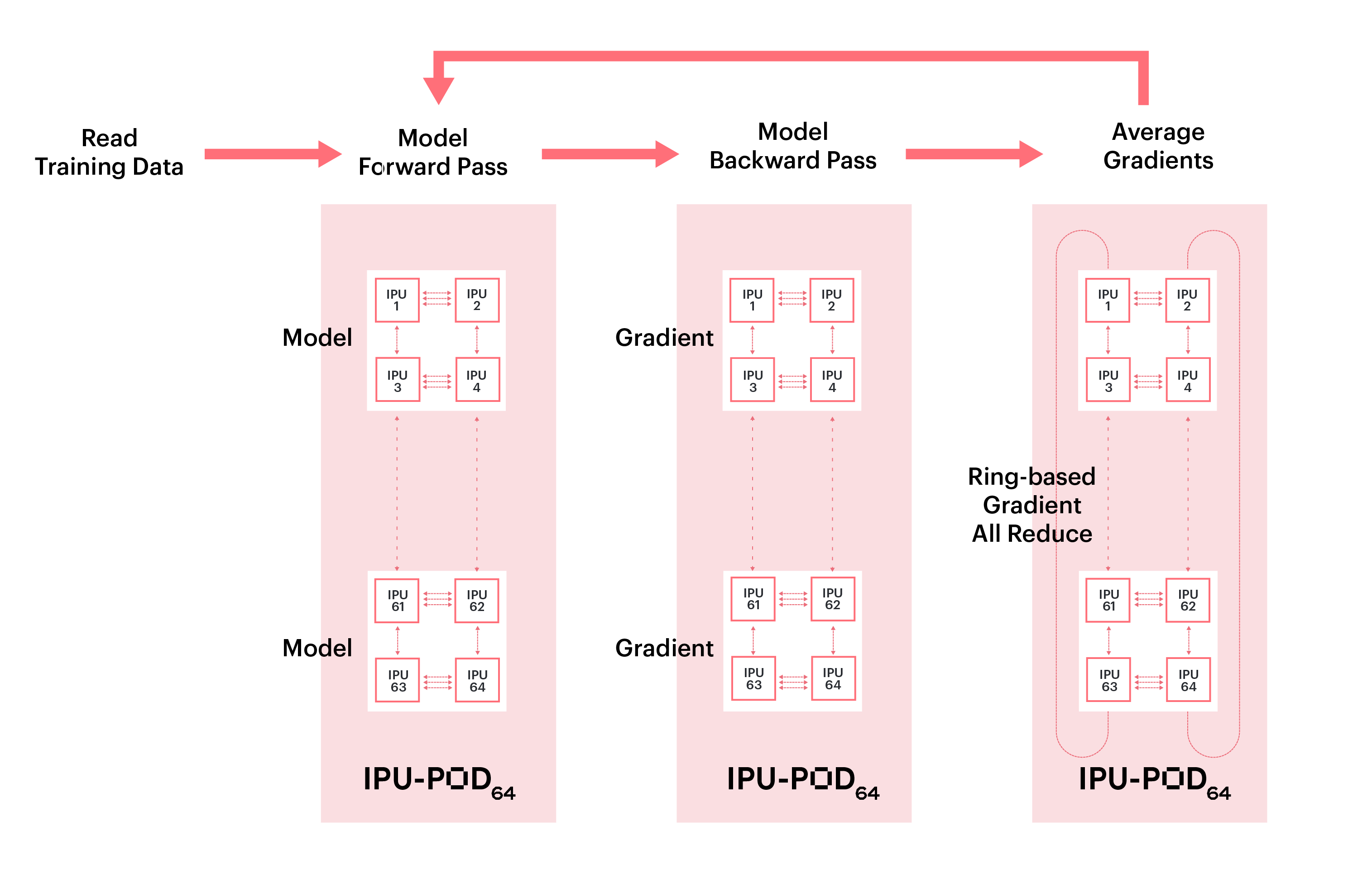
Fig. 3.1 Data parallelism for multi-replica BERT
3.2. Training BERT with large batches
One of the main contributors to the parallel scaling efficiency of the model is how frequently the gradients need to be communicated. We use gradient accumulation to decouple the compute or micro-batch size from the global batch size. This also enables us to maintain a constant global batch size when varying the number of IPUs and/or replicas by adjusting the gradient accumulation factor: global batch size = replica batch size × number of replicas. Where, replica batch size = compute batch size × gradient accumulation factor.
For a fixed number of replicas a larger global batch size therefore enables a higher GA factor and fewer optimizer and communication steps.
However, if the GA is too large, such as several thousand, this may cause underflow problems with FP16. Conversely, a small GA can lead to low pipeline efficiency due to the bubble overhead, as described in Huang et al. 2018. Some experimentation may be required to find the optimal value.
In the following sections, we will first go through some general principles for optimizing for the IPU, before looking into the layer-wise adaptive moments (LAMB) optimizer.
3.2.1. Linear scaling rule
Goyal et al. 2017 used a linear scaling rule when training large global batches for ResNet-50 and Mask R-CNN, which means that when the replica batch size \(n\) is multiplied by \(k\), (where \(k\) is usually the number of model replicas), the base learning rate, \(\eta\), should be multiplied by \(k\) and set to \(k \eta\).
Increasing global batch sizes from \(n\) to \(n k\), while using the same number of training epochs and maintaining the testing accuracy, can reduce the total training time by a factor of \(k\) and dramatically shorten the model-to-production time. However, task performance is observed to degrade with large global batches.
3.2.2. Gradual warmup strategy
One way of mitigating this is warmup, where the learning rate is not initialized as \(k \eta\) immediately. Instead, the training procedure starts with a zero, or arbitrary small, learning rate and linearly increases it over a predefined number of warmup steps until it reaches \(k \eta\). This gradual warmup enables large global batch training with many fewer steps to achieve similar training accuracy to the smaller batch size. In Goyal et al. 2017 this enabled training with a global batch size of ~8,000.
The predefined warmup steps are different for phase 1 and phase 2 in the BERT-Large pre-training case. As in the BERT paper (Devlin et al. 2018, appendix A2), our phase 1 uses training data with a maximum sequence length of 128, and a maximum sequence length of 384 for phase 2. The warmup for phase 1 is 2000 steps, accounting for around 30% of the entire training steps in phase 1. By comparison, in phase 2 there are 2100 steps in total, of which approximately 13% are for warmup.
The warmup steps may need to be tuned for different pre-training datasets.
3.2.3. AdamW optimizer
The standard stochastic gradient descent algorithm uses a single learning rate for all weight updates and keeps it constant during training. In contrast, Adam (adaptive moment estimation) makes use of the moving exponential average of the first and second moments of gradients, and adapts the learning-rate parameter based on these moments.
Loshchilov and Hutter 2017 discovered that L2 regularization is not effective in Adam, and proposed AdamW which applies weight decay regularization during the weight update step instead of L2 regularization at the loss function. This allows weights to decay multiplicatively rather than by an additive constant factor. The authors demonstrate that AdamW with warm restarts has better training loss and generalization error for both CIFAR-10 and ResNet32x32.
In IPU‑POD16 BERT pre-training, we experimented with AdamW using pre-training global batch sizes ranging from 512 to 2560, all achieving convergence to reference accuracy when fine-tuned on the SQuAD downstream task.
3.2.4. LAMB optimizer
The LAMB optimizer (You et al. 2019) is designed to overcome gradient instability and loss divergence caused by growing the batch size, enabling even larger batch sizes. LAMB uses the same layer-wise normalization concept as layer-wise adaptive rate scaling (LARS) so the learning rate is layer sensitive. However, for the parameter updates it uses the momentum and variance concept from AdamW instead.
The learning rate for each layer is calculated by:
where \(\eta\) is the overall learning rate, \(\| x \|\) is the norm of the parameters of this layer, and \(\| g \|\) is norm of the updates for the same AdamW optimizer.
This means LAMB normalizes the update and then multiplies it by \(\|x\|\) so that it will be of the same order of magnitude as the parameters of each layer, ensuring that the update makes some real change to each layer. Then the result is multiplied by the overall learning rate \(\eta\).
In LAMB, the weights and biases are considered as two separate layers because both have very different trust values and therefore should be treated with different learning rates. Biases and gamma, beta of batch-norm or group-norm are often excluded from layer adaption.
For BERT, LAMB enables global batch sizes of up to 65,536 in phase 1 and up to 32,768 in phase 2.
3.2.5. Low-precision training
During the early evolution of Deep Learning many models were trained using 32-bit precision floating-point arithmetic. Using lower precision is attractive because it enables both higher computational throughput (for IPUs, FP16 peak performance is four times higher than FP32) and reduces the size of tensors by a factor of two, reducing memory pressure and communication costs.
However, FP16 precision floating point has both lower precision and lower dynamic range than FP32. Others have proposed using FP16 for the calculation of the forward pass (activations) and backward pass (gradients) using loss scaling to manage the dynamic range of the activations and gradients, while retaining an FP32 copy of the master weights with FP32 accumulation of the weight gradients.
We implement loss scaling in a similar fashion when training with activations and gradients in FP16.
Graphcore IPUs have the capability to use stochastic rounding (Xia et al. 2020), in addition to traditional IEEE rounding modes. Stochastic rounding is based on a probability that is proportional to the proximity of a value to the upper and lower rounding bounds. Over a large number of samples this produces an unbiased rounding result.
The use of stochastic rounding allows us to keep our weights in FP16 throughout the training process with no perceptible loss of accuracy in the end-to-end training or downstream task performance.
The 1st and 2nd order moments in the optimizer are calculated and stored in FP32, and normalization is also carried out in FP32. The remainder of the operations in the training process are calculated in FP16.
4. Training results
4.1. Pre-training accuracy
Fig. 4.1 and Fig. 4.1 show the pre-training loss curves for our TensorFlow, PyTorch and PopART implementations. These demonstrate convergence to equivalent final training loss and very similar training curves. We also include training throughputs for all three model implementations on IPU‑POD16 and IPU‑POD64.
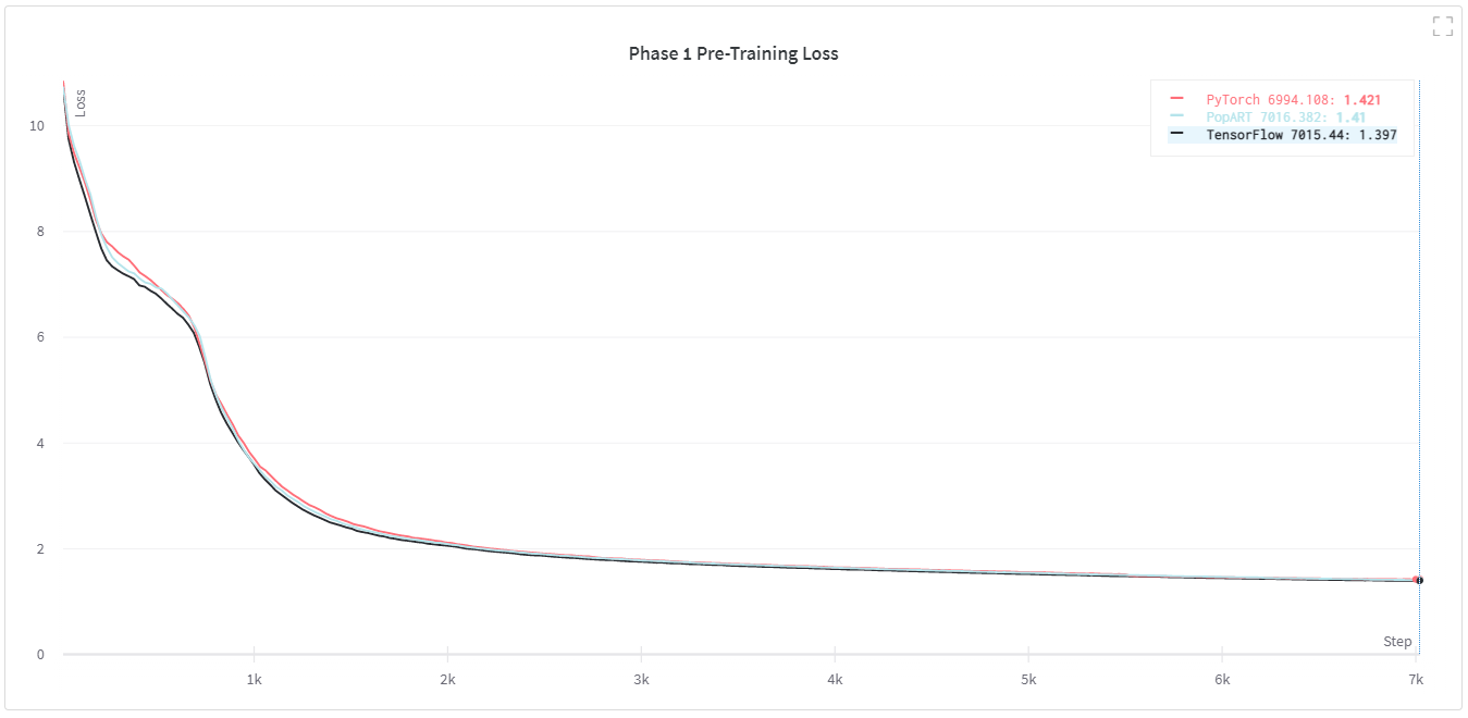
Fig. 4.1 Phase 1 pre-training loss for BERT-Large
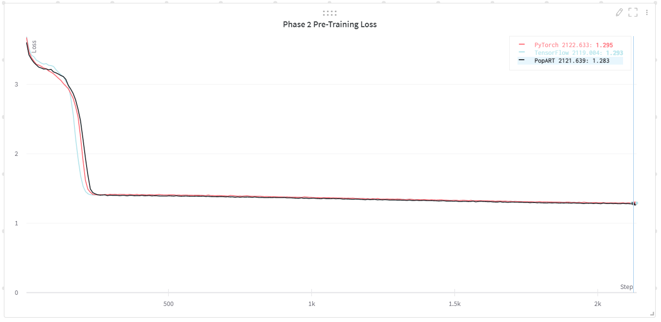
Fig. 4.2 Phase 2 pre-training loss for BERT-Large
Phase 1 throughput (S=128) (sequences/second) |
Phase 2 throughput (S=384) (sequences/second) |
|
|---|---|---|
TensorFlow |
IPU‑POD16: 3090 IPU‑POD64: 11,053 |
IPU‑POD16: 882 IPU‑POD64: 3212 |
PyTorch |
IPU‑POD16: 3525 IPU‑POD64: 12,300 |
IPU‑POD16: 979 IPU‑POD64: 3370 |
PopART |
IPU‑POD16: 3757 IPU‑POD64: 13,700 |
IPU‑POD16: 1052 IPU‑POD64: 3985 |
4.2. Fine-tuning accuracy
Once we have sufficiently trained BERT, which may need hundreds of millions of training samples, we can use these pre-trained weights as initial weights for a task-specific fine-tuning training process with a smaller amount of labelled data.
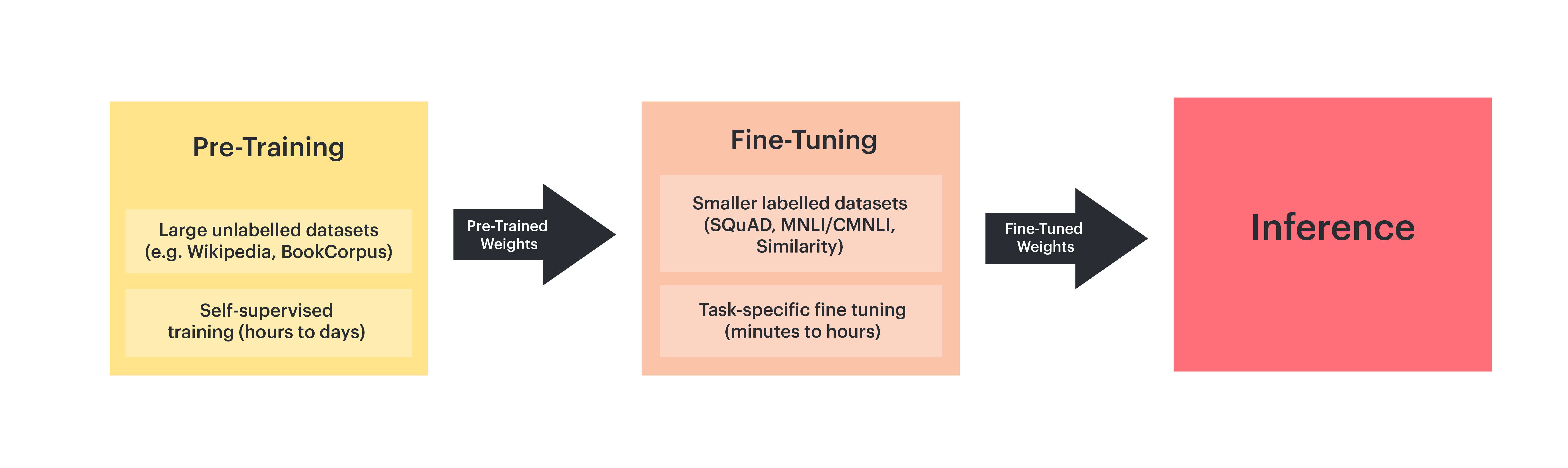
Fig. 4.3 Pre-training and fine-tuning BERT
This two-phase setup is widely used in practice because of the following advantages:
We only need to pre-train the BERT model once, for all fine-tuning tasks
Fine tuning these pre-trained models yields good task performance with less labelled data, thus saving a lot of human effort to label task-specific data
Fine-tuning can be completed in minutes or hours on an IPU‑POD4 or IPU‑POD16, depending on the size of the training dataset. Many fine-tuning trainings can be stopped after a small number of passes over the training sets.
4.2.1. SQuAD v1.1
The Stanford Question Answering Dataset (SQuAD) v1.1 is a large reading-comprehension dataset which contains more than 100,000 question-answer pairs in 500+ articles. Table 4.2 shows the accuracy when we fine-tune BERT-Large with the SQuAD v1.1 task (Rajpurkar et al. 2016) on IPUs using reference pre-trained and IPU pre-trained weights. As demonstrated, IPUs can exceed reference accuracy for this task.
BERT-Large |
Exact match |
F1 |
|---|---|---|
Reference (Devlin et al. 2018) |
84.1 |
90.9 |
IPU‑POD16 with IPU pre-trained weights |
84.5 |
90.9 |
4.2.2. CLUE
The following data shows the accuracy when we fine-tune BERT-Base with Chinese Language Understanding Evaluation (CLUE) tasks on IPUs, using Google pre-trained weights. The CLUE score is the average of the test accuracy over all the CLUE tasks, where each task’s test accuracy is the average of five experiment results. As shown in Table 4.3, IPUs can achieve the same accuracy as other AI platforms such as DGX-1 V100.
BERT-Base |
CLUE Score |
AFQMC |
TNEWS |
IFLYTEK |
CMNLI |
WSC |
CSL |
|---|---|---|---|---|---|---|---|
DGX-1 V100 |
56.55 |
72.84 |
56.59 |
59.52 |
80.28 |
63.02 |
79.89 |
Graphcore IPU‑POD16 |
56.47 |
73.33 |
56.20 |
59.31 |
79.67 |
64.09 |
79.53 |