1. Overview
The Graphcore PopLibs library includes PopSparse, a library of functions for sparse operations.
The source code is available from the Graphcore GitHub repository.
Documentation is in the Poplar and PopLibs API document.
Headers are located in the popsparse folder, APIs in the
popsparse::dynamic namespace.
The FullyConnected API (popsparse/FullyConnected.hpp) implements
matrix multiplication with a sparse operand:
Dense = Sparse * Dense
Sparse = Dense * Dense
The coordinates of elements of the sparse operand can be updated dynamically, which means during runtime and without recompilation of the Poplar Graph/Engine.
These two basic sparse matrix multiplications implement the three calculations required for a fully connected layer with back-propagation where the weights \(W\) are sparse:
Fwd: \(Y = W * X\)GradA: \(X_\textrm{grad} = W^T * Y_\textrm{grad}\)GradW: \(W_\textrm{grad} = Y_\textrm{grad} * X^T\)
By convention, in code and this document, the weights \(W\) are the
left hand operand in both the Fwd and GradA passes. Another
convention is we label the dimensions of the matrices in the Fwd
pass as follows:
\(W\) has shape \([X, Y]\)
\(X\) has shape \([Y, Z]\)
\(Y\) has shape \([X, Z]\)
When considering the three passes together, the labels for these dimensions
have the same meaning in all three passes. So, in the GradA pass:
\(W^T\) has shape \([Y, X]\)
\(Y_\textrm{grad}\) has shape \([X, Z]\)
\(X_\textrm{grad}\) has shape \([Y, Z]\)
and in the GradW pass:
\(W_\textrm{grad}\) has shape \([X, Y]\)
\(Y_\textrm{grad}\) has shape \([X, Z]\)
\(X^T\) has shape \([Z, Y]\)
Sometimes for the purposes of re-using code between passes internally,
\(X\)/\(Y\)/\(Z\) are reinterpreted in the GradA or
GradW pass as if they were a Fwd pass, so the \(X\) and
\(Y\) dimensions are swapped for GradA or the \(Z\) and
\(Y\) dimensions are swapped for GradW.
An example program that uses this API for these three passes of a fully
connected layer can be found in tools/sparse_fc_layer.cpp.
There is also a Matmul API (popsparse/Matmul.hpp) which is a thin
layer built on top of the FullyConnected API.
These APIs support element-wise (1x1 granularity) or block sparsity (4x4, 8x8, 16x16 optimised currently).
2. Background
The library was designed to meet the following requirements:
Not designed to target a particular framework’s model of sparsity (static or dynamic).
Designed originally to support the RigL optimiser (https://arxiv.org/abs/1911.11134) and other similar algorithms.
Sparsity pattern is updated during training of a neural network
Sparsity pattern is updated infrequently relative to execution of training steps, for example, once every 100 training steps
Total number of non-zero values/sparsity factor for the sparse operand is fixed (or has a known maximum)
3. Known limitations
There are certain internal restrictions on the sizes of \(X\), \(Y\), and \(Z\) dimensions that are currently not transparent to the user so they must manually pad or otherwise ensure the sizes of these dimensions meet these restrictions (an error will be thrown if not):
\(Z\) must be a multiple of 2 if
FLOATdata, and 4 ifHALFdata for element-wise sparsity (1x1 granularity).Block size in \(X\) and \(Y\) a multiple of 4 for block sparsity (anything but 1x1 granularity).
Only single-IPU is supported. This is not a fundamental limitation and multi-IPU could be supported with the same underlying algorithm in future.
Grouped matmuls are not supported, although groups are a part of the API. An error will be thrown if the number of groups is greater than 1.
4. Implementation
The implementation consists of the following key components:
lib/popsparse/FullyConnectedPlan.cpp: A planner, which searches for some optimum implementation (detailed further in Section 4.1, The Plan & Device implementation) of an operation on the device.lib/popsparse/FullyConnected.cpp: Implementation of the operation on the device based on the plan produced by the planner. This constructs the variables, compute sets, and programs needed to run the op on the device.lib/popsparse/SparsePartitioner.cpp: A host utility which encodes a sparsity pattern to be uploaded to the device and used by the device-side implementation. This uses the same plan produced by the planner to inform the encoding.
In this implementation, the host is responsible for encoding a new sparsity pattern, the result of which is uploaded to the device. In the device-side implementation, each tile reads and uses this encoded information to execute the sparse op.
4.1. The Plan & Device implementation
The plan (popsparse::fullyconnected::Plan in lib/popsparse/FullyConnectedPlan.hpp) consists primarily of a partition
between tiles (Plan::partition) and some method for computing on
each tile (Plan::method) which determines the vertices used and some
restrictions on sizes of dimensions that this method requires to work
(Method::grouping). Some other variables are part of Plan but
these mentioned are the main keys to the implementation.
Plan::partition describes how many partitions each dimension
(\(X\), \(Y\), \(Z\)) should be divided into when
calculating the result for a particular fully connected layer. All
partitions of a single dimension are of equal size except the last which
may be smaller if the number of partitions in that dimension does not
evenly the size of that dimension. For example, if \(P_X\) is the number of
partitions to divide the dimension \(X\) into, there will be
\(P_X - 1\) partitions of size
\(\left\lceil\frac{X}{P_X}\right\rceil\) and \(1\) partition of
size \(X - (P_X - 1)\left\lceil\frac{X}{P_X}\right\rceil\).
The total number of partitions is the product of the number of partitions in each dimension.
Each tile will be assigned a single partition, for which it is responsible for computing its portion of the result. This means that the number of tiles utilised is equal to \(P_\textrm{total}\). N.B. the partition is decided at compile time based on the dense matrix sizes and sparsity factor and does not change based on the specific pattern.
Method::grouping describes the dimensions of blocks that we will
divide tensors into for input/output on each tile. Vertices are written
to take inputs with the elements of these blocks contiguous in memory,
and take advantage of this to use certain instructions in the IPU
architecture. The Plan::partition partitions the tensor after it
has been divided into these groups.
4.1.1. Format of the sparse operand on the device
popsparse::SparseTensor (popsparse/SparseTensor.hpp) is the
class that represents a sparse tensor on the device. It consists of two
poplar::Tensor objects: one which contains some information encoded
by the host by SparsePartitioner (this is referred to in code as
metaInfo) and the actual values of each non-zero entry in the sparse
matrix (referred to in code as nzValues). The ordering/meaning of
these values is not exposed to the user of the library however as that
is dependent on the details of the plan chosen.
Both the metaInfo and nzValues of the
popsparse::SparseTensor are split into buckets, one of which is
mapped to each of the \(P_\textrm{total}\) tiles. Each bucket has
space for some number of nzValues and some amount of metaInfo.
The size of these buckets is set by the planner based on the sparsity
factor fixed at compile time. The encoded metaInfo and nzValues
in each bucket combined form a format similar to Compressed Row
Storage (CSR)).
Our vertices read through the metaInfo in these buckets alongside
the nzValues from the start of the bucket. The format of the
metaInfo is a sequence of integer values whose meaning is described
by the structures in lib/popsparse/SparseMetaInfo.hpp. The best way
to understand this format is by looking at the code which reads it on
each tile. As an example
lib/popsparse/codelets/SparseDenseMatMulElementWise.cpp reads the
format for element-wise sparsity (1x1 granularity).
4.1.2. Encoding a pattern and distributing non-zero values
All tiles have equal and fixed size buckets for metaInfo and
nzValues. The size is based on distributing the total/maximum number
of non-zero values for the sparse tensor across tiles evenly. So, if
\(S\) is the proportion of non-zero values in the sparse operand
(between 0 and 1) then:
where \(N_\textrm{non-zero}\) is the number of elements in
nzValues for a single bucket on a single tile — remembering that
\(P_\textrm{total}\) is equivalent to the number of tiles used
during the operation. A similar estimate is done for the size of
metaInfo for a single bucket but the CSR-style format means that the
space needed varies depending on the pattern. Because of this some extra
headroom is given in the size of these buckets which is configured using
the metaInfoBucketOversizeProportion option to the
FullyConnected API.
When a new pattern is given for encoding by SparsePartitioner, the
total number of non-zero values are distributed across the total
available space in all the buckets mapped to all tiles.
The method used by SparsePartitioner for distributing begins with
placing non-zero elements for each \(X\)/\(Y\) partition into
buckets mapped to the tiles assigned that \(X\)/\(Y\) partition
(note there are \(P_Z\) of these buckets that can contain those
values). If the buckets become full because the distribution of the
non-zero values across \(X\)/\(Y\) partitions is not uniform,
these values are ‘spilled’ to buckets on tiles assigned other
\(X\)/\(Y\) partitions.
Because the method used by SparsePartitioner to spill non-zero
elements to other \(X\)/\(Y\) partitions is not only dependent
on fitting the elements into the available space but also on reducing
the resulting runtime of the implementation on the device, we will first
describe the implementation on the device before details of
SparsePartitioner’s spilling method.
4.2. Implementation on the device
The following is a description of the algorithm which computes the result of
fullyConnectedFwd or fullyConnectedGradA using the previously
described plan and sparse tensor format. fullyConnectedGradW
is very similar in nature.
Vertices on each tile are created which have as inputs:
The slice of the dense input required to compute this partition’s result (partition in \(Y\) and \(Z\) assigned to this tile)
The bucket of the sparse tensor mapped to this tile (both
metaInfoandnzValues)
And as output:
The slice of the dense partials that will hold the results for this partition (partition in \(X\), \(Y\), and \(Z\) assigned to this tile).
The vertex is assigned a ‘sub-group ID’. We use the term sub-group to
refer to a particular \(X\)/\(Y\) partition in code. This
sub-group ID then is a single value which identifies whether a set of
non-zero values in the bucket on this tile fall within the
\(X\)/\(Y\) partition to be processed on this tile. The vertex
reads through the metaInfo skipping entries in the metaInfo and
nzValues which do not match the sub-group ID for the
\(X\)/\(Y\) partition assigned to the tile, and processing
entries which do match.
Because all partitions of \(Z\) will require the same weights as
input and because we expect SparsePartitioner to have placed as many
non-zero elements for this \(X\)/\(Y\) partition as possible
into the buckets mapped to tiles assigned this \(X\)/\(Y\)
partition, we initially execute this vertex \(P_Z\) times on each
tile unconditionally. One time to read each bucket on each tile sharing
the same \(X\)/\(Y\) partition. This step is referred to as the
‘distribution’ phase in code.
Depending how the non-zero values were distributed among buckets, the calculation may be complete at this point. If all the non-zero values for all \(X\)/\(Y\) partitions were placed in buckets on tiles assigned those same \(X\)/\(Y\) partitions then the calculation is complete.
If non-zero values were distributed to buckets assigned to tiles assigned different \(X\)/\(Y\) partitions then a further series of dynamic exchange + compute steps are executed to complete the calculation. This is called the ‘propagation’ phase. This phase is a loop:
Check against information encoded in
metaInfoto see if the calculation is complete, exit if complete.If not, exchange buckets to shift them between tiles.
Compute, dense input/output are the same but the contents of the buckets on tiles have changed.
After the distribution and propagation phases we are done with the dynamically executed steps. If \(P_Y > 1\) we have \(P_Y\) sets of partial results and one last step is added to reduce the partials to get the final result. We will not detail the final reduction as this is a dense reduction identical to that used in a dense matrix multiplication where the same dimension across which we accumulate may be partitioned across tiles.
A rough summary of all the steps is:
Distribution phase: broadcast buckets in each partition of \(Z\) to all partitions of \(Z\) and compute
Propagation phase: repeat:
Check if calculation is complete, exit if complete
Exchange buckets to shift between tiles
Compute
Reduce across \(P_Y\) if needed
The following functions build this program:
Creation of Poplar compute sets that calculate results for a partition and read sparse tensor buckets:
computefunction inFullyConnected.cpponTileImplfunction called bycomputeinFullyConnectedOnTile.cpp
Creation of copies to shift buckets between tiles:
addPropagationExchangesfunction inFullyConnected.cppwhich constructs copy programs to shift the contents of buckets between tiles.
Creation of Poplar control program that ties dynamically executed compute + exchange steps together:
ProgBuilder::addToSequencefunction inFullyConnected.cpp
4.3. Details of exchanges to shift buckets during the propagation phase
As we are creating a single static graph, we must pre-compile exchanges to move buckets between tiles. We choose to compile three sets of exchanges:
Shift buckets from each tile to the tile assigned the next partition of \(Z\) (wrapping around to 0 from the last partition)
Shift buckets from each tile to the tile assigned the next partition of \(Y\) (wrapping around to 0 from the last partition)
Shift buckets from each tile to the tile assigned the next partition of \(X\) (wrapping around to 0 from the last partition)
Because Poplar does not allow a copy to have the same memory regions as both the source and destination of a single copy as would be the case when shifting all buckets among tiles in some direction, we use two alternating buffers for buckets on each tile during the propagation phase. We maintain a flag indicating which bucket on each tile currently holds the last received/‘active’ bucket. Note that because Poplar requires our entire graph to be statically compiled, we use two sets of vertices on tiles when computing as a result of this double-buffering. One set processes each buffer, and a switch statement selects the vertices to execute based on which is ‘active’.
Due to the double buffering of buckets we actually compile six exchanges in total for these three possible directions in which to shift buckets, one with each of the two buffers as the source/destination.
4.4. Details of vertices
So far we have only described how a vertex mapped to a particular tile is responsible for computing the result for a particular partition. Here we give some details of specific hardware features used to compute within a single tile.
4.4.1. Element-wise sparsity (1x1 granularity)
For element-wise sparsity, concerning ourselves with the innermost loop
of our Fwd pass vertex’s compute, we will continuously load the
\(Y\) coordinates for the elements in the sparse operand and load
the relevant input data from the dense operand. The sparse element must
then be multiplied with each element of the dense operand in the
dimension \(Z\). This loop is done for all sparse elements with the
same \(X\) coordinate, accumulating the results, before finally
storing that result to the right \(X\) coordinate for the sparse
elements. In order to iterate sparse elements with the same \(X\)
coordinate, the coordinates are sorted during encoding by
SparsePartitioner.
As a reference the assembly for the vertex handling element-wise
sparsity for the Fwd pass with float input data/float partials can
be found in
lib/popsparse/codelets/asm/SparseDenseMatMulElementWise_float_float.S.
For loading both a \(Y\) coordinate, and 64-bits of dense input data
in a single cycle, the ldd16a64 instruction is used. See the
the Tile Vertex Instruction Set Architecture for Mk2 IPUs for full details, but in this case we use this instruction
to:
Load a 64-bit value from the dense input at a \(Y\) coordinate encoded as a 16-bit byte offset.
Load a new 16-bit \(Y\) coordinate for the next 64-bit value in the dense offset * Advance the pointer for loading \(Y\) coordinates for the iteration after that.
The non-zero value from the sparse operand is simply loaded separately
with ld32step.
For multiply-accumulating we use either f32v2mac or f32v2mul and
f32v4acc instructions depending on the vector width available to us.
The only way to take advantage of instruction-level parallelism in this
case is via the \(Z\) dimension of the dense input operand, hence
the restrictions on \(Z\) being a multiple of 2 or 4 depending on the
data type.
If \(Z\) a multiple of 2, we can achieve two MACs in two cycles using
f32v2mac.If \(Z\) is a multiple of 4, we can achieve four MACs in three cycles using
f32v2mul/f32v4acc.
For assembly of the half input data/float partials equivalent of the
above see
lib/popsparse/codelets/asm/SparseDenseMatMulElementWise_half_float.S:
If \(Z\) is a multiple of 4, we achieve four MACs in two cycles using
f16v4mulandf16v4accIf \(Z\) is a multiple of 8, we achieve eight MACs in three cycles using
f16v4mulandf16v8acc.
Note that the precision of the intermediate after the multiply is still half and not float. There is no fused multiply-accumulate instruction implemented for half in the current IPU hardware that could give the true float partial type for the calculation, and so this is a compromise as performance without it would be much worse due to need to cast inputs up to float precision.
4.4.2. Block sparsity (anything but 1x1)
For block sparsity there is much more work to do for each coordinate in the input buckets. We have specialised vertices for 4x4, 8x8, and 16x16 block sizes.
These vertices all utilise the IPU’s AMP units which are designed specially to perform matrix multiplication. Here blocks are loaded into weight memory for the AMP unit, and vertices iterate over the \(Z\) dimension of the dense input multiplying with the currently loaded block from the sparse operand.
4.4.3. Vertex specialisations
You may note there are many vertices in lib/popsparse/codelets that
go beyond just element-wise/block sparsity. We will briefly describe the
reasons for having some of these:
...GradW: As theGradWpass has a different sparse operand (the output) the code needs specialising for this case always.SparseDenseMatMulGradWElementWise: GradW for element-wise sparsity, inner loop is now accumulating over \(Z\). Some code paths specialise to improve vertex runtime for small values of \(Z\) (2, 4 or 8 depending on input data/partials types).SparseDenseMatMulBlockAmpGradW: utilises AMP hardware, but requires a transposition of dense inputs from theFwd/GradApasses. Because of the need to transpose, depending on size/shape of the problem it may be faster to use the alternative:SparseDenseMatMulBlockGradW: does not utilise AMP hardware and so has lower maximum throughput but does not require a transposition of inputs from theFwd/GradApasses.
SparseDenseMatMulBlockGradA: Where possible we want to re-use themetaInfodescribing non-zero values between passes. In theGradApass the \(X\)/\(Y\) coordinates are essentially swapped and so to use the samemetaInfoas for theFwdpass we must specialise the code to read themetaInfointerpreting the coordinates differently.SparseDenseMatMulGradAElementWise: This specialisation is almost identical toSparseDenseMatMulElementWiseused for the forward pass. The difference is that themetaInfooffsets into to the samenzValuesin the same order in memory as they were for theFwdpass and so thismetaInfofor theGradApass both has transposed coordinates and includes coordinates for the weights in the transposed order alongside the coordinates used to load the dense input operand. We need the second set of offsets for weights in order to iterate in the new transposed order.SparseDenseMatMulElementWiseTranspose: As withSparseDenseMatMulBlockGradAthis is a version of the element-wiseGradAvertex that re-usesmetaInfofrom theFwdpass. The coordinates are transposed on the fly. There is a trade off between size ofmetaInfoand speed of execution here in that for element-wise sparsity in-particular transposing the coordinates on the fly is very slow because the same inner-loop accumulating over sparse elements with the same \(X\) coordinate is not possible.
4.5. Performance characteristics
The best case scenario for a matrix multiplication with this algorithm is when non-zero values in the sparse operand are evenly spread among \(X\)/\(Y\) partitions.
Each tile does an equal share of the total FLOPs for the operation.
In this case, the buckets mapped to tiles assigned each \(X\)/\(Y\) partition should have space enough to hold all non-zero values falling within that \(X\)/\(Y\) partition. As all the non-zero values are in the buckets assigned to the tiles that must process them, we can complete the operation in the distribution phase and no further exchange + compute steps are needed.
In the examples in Fig. 4.1 and Fig. 4.2, \(P_Z = 1\), greater values of \(P_Z\) simply distribute the FLOPs in each \(X\)/\(Y\) partition evenly among \(P_Z\) tiles.
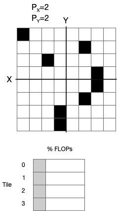
Fig. 4.1 Best case scenario
The worst case scenario is when all non-zero values in the sparse operand lie within a single \(X\)/\(Y\) partition.
The tile(s) assigned to the \(X\)/\(Y\) partition in which all the non-zero values lie must do all the FLOPs for the operation, and all the other tiles do no useful work.
In this case, all the non-zero elements must be spread between all the buckets because the size of the buckets mapped to the tile(s) processing the partition of \(X\)/\(Y\) with all the non-zero elements is only big enough to contain \(1/P_\textrm{total}\) of the elements (unless bucket size was increased manually via options). This means that we must exchange + compute somewhere up to \(P_\textrm{total}\) times to complete the operation.
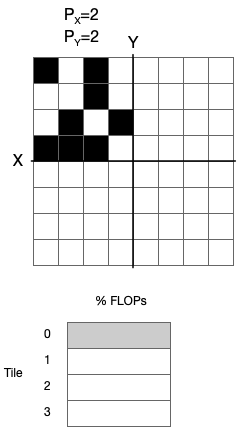
Fig. 4.2 Worst cast scenario
4.6. SparsePartitioner spilling method
Somewhere in-between the two extremes described, there is a choice about how to spill non-zero elements from buckets which become too full (due to non-uniform distribution of sparsity pattern) to other buckets. We can now describe this.
The propagation phase uses the three sets of exchanges compiled into the program to shift buckets in each direction along partitions of \(X\), \(Y\), and \(Z\) in a nested loop. In order of innermost to outermost loop buckets are cycled around partitions of \(Z\), then \(Y\), then \(X\).
When choosing a bucket to spill elements to when buckets mapped to tiles assigned those elements’ \(X\)/\(Y\) partition are full, we can define a concept of a kind of distance based on this nested iteration and attempt to minimise this distance for all elements. We can use the number of compute steps required as this distance. For example elements in buckets mapped to tiles assigned the \(X\)/\(Y\) partition they fall within are at distance \(P_Z\). \(P_Z\) is the minimum distance because all partitions of \(Z\) must all process the same weights and in the best case scenario these weights are spread over \(P_Z\) buckets. Elements in buckets mapped to tiles assigned the previous \(Y\) partition than that they fall within are at distance \(2P_Z\) as we must calculate \(P_Z\) times, then shift once in the \(Y\) direction, then shift \(P_Z\) times again and so on.
SparsePartitioner attempts to minimise this concept of distance for
all elements by spilling elements from buckets first to buckets mapped
to tiles assigned consecutive previous partitions of \(Y\), then
consecutive previous partitions of \(X\) and so on.
4.7. GradW pass
The above implementation descriptions primarily described details of
fullyConnectedFwd/fullyConnectedGradA passes.
In the GradW pass it is the output that is the sparse operand and
both inputs are dense. The algorithm is largely the same but code is
specialised. nzValues buckets are partials that vertices
continuously sum into until the computation is complete. Buckets are
similarly cycled around tiles when elements were spilled by
SparsePartitioner and all the same concepts apply.
4.8. Planning
We plan jointly for all three passes (called Fwd, GradA, and
GradW in this library), or whichever passes are present in a
particular network/program as indicated by options to the operation
doGradAPass/doGradWPass (Fwd is assumed to always be
present). Most importantly the same partition is used to implement all three
passes here, with dimensions appropriately swapped depending on the
pass.
Planning jointly means we produce a plan attempting to minimise some
cost across execution of all passes that will be executed. We attempt
to minimise an estimated cycle count to compute in each pass, including
data movement between and during passes (such as
transposition/exchange). Memory usage is also controllable via an option
availableMemoryProportion which controls the maximum proportion of
tile memory that should be used by the operation for temporary memory.
To obey this limit we also estimate temporary memory usage of the
operation.
The planner currently assumes a totally unstructured sparsity pattern,
where we don’t know anything about the sparsity patterns that will arise
during training. As a result, the planner optimises for the previously
described best case scenario, where we only need a single step of
compute to complete the whole operation. Temporary memory for any
further steps of exchange + compute is still estimated and contributes
to the memory usage estimates that are needed for
availableMemoryProportion.
Planning utilises an integer constraint solving library in poplibs
called popsolver to declare relationships between variables such as
the number of partitions of \(X\)/\(Y\)/\(Z\) and the total
estimated cycles and then to minimise the value of the estimated cycles.
popsparse::fullyconnected::getPlan in FullyConnectedPlan.cpp is
the top-level entry point for the planner.