8. Graphs

8.1. Main graph

You can create the main graph of an IR by calling main_graph. The returned main graph can be used as a context to include its operations and tensors.

8.2. Graphs

You can create a subgraph (Section 2.2, Graphs) in PopXL by calling, for example, create_graph(). You then connect the subgraph with the calling graph with the call() op. In PopXL, you have access to create_graph() before you call a graph with call(), which gives you the flexibility to manipulate the graph.

Listing 8.1 shows a basic example for how to create and call subgraphs. In the example, a subgraph is created and called instead of directly calling the Python function increment_fn().

Listing 8.1 Example to create and call graphs

def increment_fn(x: popxl.Tensor):
    return x + np.ones(x.shape, x.dtype.as_numpy())


with main:
    # host load
    input = popxl.h2d_stream([2, 2], popxl.float32, name="input_stream")
    x = ops.host_load(input, "x")

    # create graph
    increment_graph = ir.create_graph(increment_fn, x)

    # call graph
    (o,) = ops.call(increment_graph, x)

Download basic_graph.py

8.3. Creating a graph

You can create a subgraph by calling the function create_graph(). You can use the same function to create multiple subgraphs. In the example in Listing 8.2, two different graphs are created for different input tensors, w1 and w2, which have different shapes.

Listing 8.2 Example of creating multiple graphs with same function

def matmul_fn(x: popxl.Tensor, w: popxl.Tensor):
    return x @ w


with main:
    # host load
    input = popxl.h2d_stream([2, 2], popxl.float32, name="input_stream")
    x = ops.host_load(input, "x")

    w1 = popxl.variable(np.ones(x.shape, x.dtype.as_numpy()), name="w1")
    w2 = popxl.variable(np.ones(x.shape[-1], x.dtype.as_numpy()), name="w2")

    # create two graphs
    matmul_graph1 = ir.create_graph(matmul_fn, x, w1)
    matmul_graph2 = ir.create_graph(matmul_fn, x, w2)

Download create_multi_subgraphs_from_same_func.py

You can also create the subgraph with an additional graph input with graph_input() in its Python function. graph_input() creates a new input tensor for the subgraph. An example can be found in Listing 8.3.

8.4. Calling a graph

After you have created a subgraph, you can invoke it with call(). The input tensors are as follows:

call(graph: Graph,
    *inputs: Union[Tensor, List[Tensor]],
    inputs_dict: Optional[Mapping[Tensor, Tensor]] = None
    ) -> Union[None, Tensor, Tuple[Tensor, ...]]:

inputs are the inputs the subgraph requires and they must be in the same order as in create_graph(). If you are not sure about the order of the subgraph internal tensors that are defined by graph_input(), you can use inputs_dict to provide the mapping between the subgraph tensors and the parent graph tensors.

Listing 8.3 shows an example of a graph being called multiple times with different inputs. In this example, the subgraph was created with an additional graph input value. When you call this subgraph, you will have to pass a tensor to the subgraph for this input as well. You can use it to instantiate the weights of layers internally.

Listing 8.3 Example of a graph being called multiple times with different inputs

def increment_fn(x: popxl.Tensor):
    value = popxl.graph_input(x.shape, x.dtype, "value")
    return x + value


with main:
    # host load
    input = popxl.h2d_stream([2, 2], popxl.float32, name="input_stream")
    x = ops.host_load(input, "x")

    # create graph
    increment_graph = ir.create_graph(increment_fn, x)

    # two variable values
    value1 = popxl.variable(np.ones(x.shape, x.dtype.as_numpy()), name="value1")
    value2 = popxl.variable(2 * np.ones(x.shape, x.dtype.as_numpy()), name="value2")

    # call graph
    (o,) = ops.call(increment_graph, x, value1)
    (o,) = ops.call(increment_graph, o, value2)

Download multi_call_graph_input.py

Instead of calling a graph with call(), you can call it and get the information about the call site with the op call_with_info(). This op returns a CallSiteInfo object that provides extra information about the call site. For instance, you can get the graph being called using called_graph. inputs and outputs return the input tensors and output tensors respectively. You can also obtain the input and output tensors at a given index with parent_input(index) and parent_output(index) respectively. You can find the input graph tensor that corresponds to a parent tensor using parent_to_graph (parent_tensor). graph_to_parent(graph_tensor) provides an input or output tensor in called_graph that associates the input or output tensor in the parent graph.

With the CallSiteInfo object, you can use set_parent_input_modified(subgraph_tensor) to specify that the input tensor subgraph_tensor can be modified by this call_with_info() op. This provides support for in-place variable updates as in Listing 8.4. After calling the subgraph, the value of the variable tensor x is changed to 2.

Listing 8.4 Example of call_with_info op

def increment_fn(x: popxl.Tensor):
    value = popxl.graph_input(x.shape, x.dtype, "value")
    # inplace increment of the input tensor
    ops.var_updates.copy_var_update_(x, x + value)


with main, popxl.in_sequence():
    x = popxl.variable(1)
    value1 = popxl.constant(1)

    # create graph
    increment_graph = ir.create_graph(increment_fn, x)
    # call graph
    info = ops.call_with_info(increment_graph, x, value1)
    info.set_parent_input_modified(x)
    # host store
    o_d2h = popxl.d2h_stream(x.shape, x.dtype, name="output_stream")
    ops.host_store(o_d2h, x)

Download call_with_info.py

The op call_with_info() is helpful when building and optimizing the backward graph. More details are given in Section 9.1, Autodiff.

8.5. Calling a graph in a loop

You can use the op repeat() to create a loop.

repeat(graph: Graph,
       repeat_count: int,
       *inputs: Union[Tensor, Iterable[Tensor]],
       inputs_dict: Optional[Mapping[Tensor, Tensor]] = None
       ) -> Tuple[Tensor, ...]:

This calls a subgraph graph for repeat_count number of times. Its inputs are:

• inputs denotes the inputs passed to the subgraph function and,

• inputs_dict denotes a mapping from internal tensors in the subgraph being called to tensors at the call site in the parent graph.

Both inputs from inputs and inputs_dict are “loop-carried” inputs. This means that they are copied into the subgraph as inputs before the first iteration is run. The outputs of each iteration are copied to the inputs of the next iteration as shown in Fig. 8.1. The outputs of the last iteration serve as the outputs of the repeat() op.

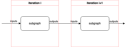
Fig. 8.1 Repeat op graph

The repeat() op requires that the number of the subgraph inputs, including the inputs and the inputs_dict, to be at least the number of outputs.

Note

This operation requires the repeat count to be greater than 0.

In Listing 8.5, the graph increment_graph from increment_fn is called twice. The input x is incremented twice by value. After the first iteration, the outputs x + value and value are copied to the inputs for the second iteration.

Listing 8.5 Example of repeat op to increment a tensor by a fixed value

def increment_fn(x: popxl.Tensor, value: popxl.Tensor):
    return x + value


with main:
    # host load
    x = popxl.variable(np.ones([2, 2], np.float32), name="x")
    value = popxl.variable(np.ones(x.shape, x.dtype.as_numpy()), name="value")

    # create graph
    increment_graph = ir.create_graph(increment_fn, x, value)

    # call graph in a loop
    (o,) = ops.repeat(increment_graph, 2, x, value)

Download repeat_graph_0.py

Listing 8.6 shows how to use the inputs_dict. The callable class Linear defines a linear layer. The subgraph linear_graph is created from the PopXL build method.

Listing 8.6 Example of repeat op using inputs_dict

class Linear(popxl.Module):
    def __init__(self):
        self.W: popxl.Tensor = None
        self.b: popxl.Tensor = None

    def build(
        self, x: popxl.Tensor, out_features: int, bias: bool = True
    ) -> Tuple[popxl.Tensor, ...]:
        self.W = popxl.graph_input((x.shape[-1], out_features), popxl.float32, "W")
        y = x @ self.W
        if bias:
            self.b = popxl.graph_input((out_features,), popxl.float32, "b")
            y = y + self.b
        return y


with main:
    # host load
    x = popxl.variable(np.ones([2, 2], np.float32), name="x")
    W = popxl.variable(np.ones([2, 2], np.float32), name="W")
    b = popxl.variable(np.ones([2], np.float32), name="b")

    # create graph
    linear = Linear()
    linear_graph = ir.create_graph(linear, x, out_features=2)

    # call graph in a loop
    # the x, W, b will be copied to the input of the `linear_graph` before the first iteration
    # the outputs of each iteration will be copied to the inputs of the next iteration
    # The outputs of the last iteration serve as the output of the `repeat` op
    (o,) = ops.repeat(linear_graph, 2, x, inputs_dict={linear.W: W, linear.b: b})

Download repeat_graph_1.py

8.6. Graph replication

For improved performance, multiple IPUs can run in data parallel mode. In data parallel mode multiple replicas of the graph are run on separate sets of IPUs.

Replicas can be grouped, see Section 13, Replication. By default, there is only one group. Replicas in a group are loaded with the same values.

Most operations can use replica grouping to reduce over only the grouped replica graphs, allowing for all replicas in a group to benefit from each other’s updates.

Graph replication cannot be used with IPU Model targets.

To set the replication factor (the number of replicated graphs), you can set the ir.replication_factor.

8.7. Code loading from Streaming Memory

By default, tile memory is required for the tensors in the graph and for the executable code for the compiled graph. To help alleviate this memory pressure, as with tensors, you can store the executable code in Streaming Memory and load it, when required, back into executable memory on the tiles.

Note not all the code will be offloaded and re-loaded. For example, Poplar will decide whether mutable vertex state or global exchange code will remain always live. The code that is not offloaded will just stay in executable memory, and executing the graph will always work without the requirement to explicitly load those parts of code onto the IPU.

8.7.1. Minimal example

In PopXL, this code loading happens at the granularity of Graph objects, because it is each Graph that is compiled into one or more poplar::Function objects, which is then compiled into executable IPU code.

A minimal example follows:

Listing 8.7 Minimal example of code loading in PopXL

    with ir.main_graph:
        # (1) insert many ops ...

        with popxl.in_sequence():
            # (2) load the code from remote memory into compute tiles on-chip
            ops.remote_code_load(g, destination="executable")
            # call the graph
            ops.call(g, x)

            # insert more ops...

            # call the graph again
            ops.call(g, x)

            # (3) call the graph for the final time
            ops.call(g, x)

Download code_loading.py

From the example, you can see that no remote buffer for the Graph code is explicitly created by the user. Instead, the ops.remote_code_load() for that graph from Streaming Memory tells PopXL to create that remote buffer implicitly for you. Multiple ops.remote_code_load calls from Streaming Memory on the same Graph will reuse the same remote buffer. Note it is your responsibility to remember to insert the remote_code_load op, otherwise it will seem to PopXL that the user intends to have the code always-live in executable memory as normal. The in_sequence() context around the remote_code_load and call is also mandatory to ensure the copy is scheduled before the call. The need for this is explained later. The other possible values of the parameter destination are also explained later.

In the above example, all the ops and tensors will be lowered into Poplar as usual, then the Poplar liveness analyser will try to minimise liveness across the computation by reusing memory where available. In this case, the liveness analyser will see that the code does not need to be live until the remote_code_load call. Therefore the code is “dead” from (1) until (2), and hence less memory is consumed during this time. After the remote_code_load, the code is considered live. We can call the Graph (that is, execute the code) as many times as we want — the code is still on device. At (3), we call the Graph for the final time. The Poplar liveness analyser may use this fact to consider the code dead after this point, and again recycle that memory for another use.

To summarise, the code is only live from (2) to (3), whereas without code loading, the code would have been always-live.

Note that when we say the code is “dead” or “not live”, it is not guaranteed that the memory will indeed be reused for something else, only that it could be. Any part of the compilation stack may choose to optimise the graph in a different way instead if it believes doing so to be more beneficial.

Lastly, the fact that the remote_code_load and call are inside an in_sequence context is very important. Recall that, in PopXL, you are building a data-flow graph of ops and tensors, and by default they will execute in whatever order the internal scheduler decides best (it aims to minimise liveness). Observe that there is no data-flow dependence between the remote_code_load and the call, meaning there is no tensor that the remote_code_load produces that the call consumes. This means, without the in_sequence, they could be scheduled in any order, and if the call comes first, the Poplar liveness analyser will think the code needs to be always-live (in the case of the above example). Therefore, failing to use in_sequence results in undefined behaviour with respect to the code liveness, and the onus is on you to remember to use it.

8.7.2. Controlling liveness between multiple calls

Every time you call a graph, it signifies that the code should be in tile executable memory since either the last remote_code_load(destination='executable'), or if there is no previous remote_code_load(destination='executable'), the start of the program, in other words the code is always-live.

Every time you use remote_code_load to load a Graph into a location, it signifies that the code did not need to be live in that location since the last call, or if there is no previous call, from the start of the program.

Together, this gives full control of the code liveness of your graphs. Say you have repeated calls to a Graph and you want the code to always be dead in between calls until the latest possible moment. You simply insert remote_code_load ops just before every call. The following example demonstrates this:

Listing 8.8 Code loading example with multiple loads and calls

    with ir.main_graph:
        with popxl.in_sequence():
            # Dead...

            # Live
            ops.remote_code_load(g, destination="executable")
            ops.call(g, x)

            # Dead again, due to a subsequent load...

            # Live again
            ops.remote_code_load(g, destination="executable")
            ops.call(g, x)

            # Dead again, due to a subsequent load...

            # Live again
            ops.remote_code_load(g, destination="executable")
            ops.call(g, x)

            # Dead again, as graph never called again

Download code_loading.py

Note in the example we do not copy back the code from device to Streaming Memory. This is for two reasons. Firstly, the code has no mutable state, so it is valid to just keep loading repeatedly from the same remote buffer. In Poplar, it is possible for code to have “mutable vertex state”, but currently Poplar will never offload that part of the code anyway and keep it always-live. Secondly, Poplar attempts no liveness analysis in Streaming Memory to reuse a buffer for something else when it is not needed. If this were the case, copying the code to device would effectively free that space in Streaming Memory; so since that space cannot be reused, it is pointless to perform the copy. Therefore, there is no API for copying code to Streaming Memory.

8.7.3. Optimisation: merging the code load operations

Poplar will attempt to merge exchanges of code data just like with other remote buffer copies. That is, if you are loading code for multiple graphs, and if there are no ops that cause a global exchange between the load ops in the schedule (which you can ensure is the case using in_sequence), then Poplar will merge the exchanges for those loads, resulting in a speed-up. In PopXL, it is up to you to decide if this is beneficial for your use-case and impose such a schedule using in_sequence().

Secondly, again as with regular tensors, careful scheduling of the ops can ensure the IO of the code loading overlaps with computation. Though we cannot give a full exposition of overlapped IO here, the basics are as follows: if you want IO A to overlap with compute B:

• A must come before B in the schedule.

• There can be no data-dependency between A and B.

• A must be placed on IO tiles.

• B must be placed on compute tiles.

• If A consists of multiple stream copies, they must be adjacent in the Poplar sequence so that they are mergeable.

8.7.4. Advanced example: nested code loading

To help us further understand the semantics of code loading, let’s examine a nested example where we use remote_code_load to load a graph that uses remote_code_load to load another graph:

Listing 8.9 Example of nested code loading

    def expensive_id(x: popxl.Tensor) -> popxl.Tensor:
        return x.T.T

    g1 = ir.create_graph(expensive_id, x.spec)

    def load_g1():
        ops.remote_code_load(g1, destination="executable")

    g2 = ir.create_graph(load_g1)

    with ir.main_graph, popxl.in_sequence():
        # Loads code for g1
        ops.remote_code_load(g1, destination="executable")

        # Loads code for g1
        ops.call(g2)

        # Execute g1
        ops.call(g1, x)

Download code_loading.py

In this example, calling g1 performs the load for g2. After this, we can now execute g2 on device.

We could also change the load_g1 function to instead take the Graph as a parameter, then dynamically make many graphs for loading the code of other graphs. Note however that the graph that performs the loading cannot dynamically load any graph — it is fixed to a certain graph on creation. Only the function load_graph for creating such a Graph is dynamic and can be reused for creating many graphs:

Listing 8.10 More complex example of nested code loading

    def load_graph(g: popxl.Graph):
        ops.remote_code_load(g, destination="executable")

    g3 = ir.create_graph(load_graph, g1)
    g4 = ir.create_graph(load_graph, g2)

    with ir.main_graph, popxl.in_sequence():
        ops.remote_code_load(g3, destination="executable")
        ops.call(g3)

        ops.remote_code_load(g4, destination="executable")
        ops.call(g4)

Download code_loading.py

8.7.5. Advanced concept: code loading in dynamic branches

Graphs can have dynamic branching in them, for example through an if op. Say there are ops.remote_code_load ops in these dynamic branches, what effect will this have on the liveness of that code?

Liveness analysis is a static compile-time concept. We do not know which branch will be taken at runtime. Say we perform the remote_code_load op in only one of the branches, then call the graph after the branches merge again (so after the if op). At the point of the call, the compiler does not know if the remote_code_load will have happened or not, as it does not know which branch will be taken at runtime. The compiler has to produce a program that accounts for all possible cases, so it must pessimistically plan as if the remote_code_load did not happen. Therefore, it will assume the code was already live on the device before the branching.

Essentially, if there is branching before a call, only if all possible branches contain a remote_code_load can we assume that the code was dead and in Streaming Memory until the remote_code_load op. If any possible branch does not perform a remote_code_load, we must assume that there was no remote_code_load and the code was already live before the branching.