3. ResNeXt inference example

When being introduced to a new API, it is often helpful to have a working example of code to get a general overview of the key elements involved. A particular model which is useful to review given its simple, but non-trivial topology is ResNeXt.

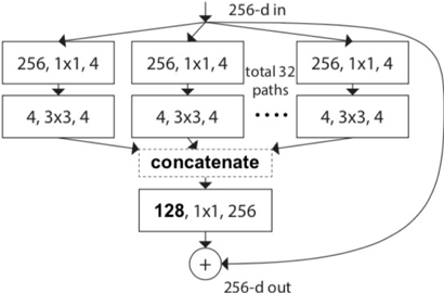
ResNeXt is an Inception inspired model based on ResNet with repeated computational blocks interspersed with residual connections. Its primary distinguishing characteristic is the use of group convolutions in its module compute structure. Group convolutions, as opposed to conventional convolutional layers, partition the output channels of the operation into segregated groups. The number of segregated groups is referred to as the model’s cardinality, which the authors state allows for more robust syntax extraction by allowing for more complex transformations. An illustration of cardinality is given in Fig. 3.1 below, where each of the [256, 1, 1, 4] streams in the graph represent a distinct convolution set, while the structure as a whole is a group convolution.

Fig. 3.1 ResNeXt cardinality expressed via group convolutions. Refer to Xie (2017) for more details.

3.1. Abridged sample code

In the code sample that follows, only those facets that are specific to the IPU API are explicitly documented, while other general items of TensorFlow development are identified but mostly omitted. A full working version of the code can be found in Section 7, ResNeXt full code example. Omissions are indicated by … and accompanied by comments to define the nature of what has been redacted.

import tensorflow as tf
... # Various additional import statements

# Import IPU API
from tensorflow.python import ipu

# Create a dataset for in-feed interface into session call
def create_input_data(batch_size=1, height=224, width=224, channels=4):
    # Synthetic input data follows NHWC format
    input_data = np.random.random((batch_size, height, width, channels))
    input_data = tf.cast(input_data, DTYPE)

    ds = tf.data.Dataset \
        .range(1) \
        .map(lambda k: {"features": input_data}) \
        .repeat() \
        .prefetch(BATCHES_PER_STEP).cache()
    return ds

... # Various layer wrappers required by model definition,
    # (e.g. convolution, max pool)

# Group convolution definition
def group_conv(x, ksize, stride, filters_in, filters_out, index=0, groups=1,
               dtype=tf.float16, name='conv'):
    with tf.variable_scope(name, use_resource=True):
        # Define a weight variable
        W = tf.get_variable("conv2d/kernel" + str(index),
                            shape=[ksize, ksize,
                                   filters_in.value / groups,
                                   filters_out], dtype=dtype,
                                   trainable=True,
                                   initializer=tf.variance_scaling_initializer())
        # Implicit group convolution since channels of W are fraction of x
        return tf.nn.conv2d(x, filters=W, strides=[1, stride, stride, 1],
                             padding='SAME')

def group_conv_block(x, first_stride, filters, count, name='', cardinality=4):
    ... # Define the modular group convolution block as described in the paper
    return x

# Define the ResNext model
def resnext101_model():
    def body(features):
        with tf.variable_scope("VanillaResNeXt"):
            ... # Elements of model definition
            output = fc(x, num_units_out=1000)
            outfeed = outfeed_queue.enqueue(output)
            return outfeed
    return tf.python.ipu.loops.repeat(n=BATCHES_PER_STEP, body=body,
                                     infeed_queue=infeed_queue)

if __name__ == '__main__':
    # no simulation
    IPU_MODEL = False

    ... # Various additional variables

    # Create input data using randomized numpy arrays
    dataset = create_input_data(batch_size=BATCH_SIZE, height=224, width=224, channels=4)

    if IPU_MODEL:
        os.environ['TF_POPLAR_FLAGS'] = "--use_ipu_model"

    # Setup infeed queue
    with tf.device('cpu'):
        infeed_queue = ipu.ipu_infeed_queue.IPUInfeedQueue(dataset,
                                             feed_name="inference_infeed")

    # Setup outfeed
    outfeed_queue = ipu.ipu_outfeed_queue.IPUOutfeedQueue(feed_name="outfeed")

    # Compiles graph and targets IPU(s)
    with ipu.scopes.ipu_scope('/device:IPU:0'):
        res = ipu.ipu_compiler.compile(resnext101_model, inputs=[])

    # Setup IPU configuration and build session
    cfg = ipu.config.IPUConfig()
    cfg.convolutions.poplar_options["availableMemoryProportion"] = "0.3"
    cfg.auto_select_ipus = 1
    cfg.configure_ipu_system()
    ipu.utils.move_variable_initialization_to_cpu()
    outfeed = outfeed_queue.dequeue()

    # Create a session initiation and run the model
    with tf.Session() as sess:
        fps = []
        latency = []
        sess.run(infeed_queue.initializer)
        sess.run(tf.global_variables_initializer())
        # Warm up
        print("Compiling and Warmup...")
        start = time.time()
        sess.run(res)
        outfeed = sess.run(outfeed)
        for iter_count in range(NUM_ITERATIONS):
            print("Running iteration for benchmarking: ", iter_count)
            sess.run(res)
            sess.run(outfeed)
            ... # Various summary statistics

In the following three sections, we review specific elements of the code presented, using the line numbers to identify the pertinent code elements.

3.2. Preliminaries: getting up and running

Before running the script, it is necessary to ensure a Poplar SDK has been downloaded and extracted (for more information see the Getting Started guide for your IPU system) on an IPU-enabled platform and that the environment variables are set appropriately.

# Export statements
export TMPDIR=/mnt/data/username/tmp/
export TF_POPLAR_FLAGS="--executable_cache_path=/mnt/data/username/ipu_cache/"
export POPLAR_LOG_LEVEL=INFO

Moving on to the export statements, Poplar and TensorFlow’s XLA backend, both cache parts of the compilation to speed up graph construction. It is important to make sure there is enough space for it, which is why the first export statement points to a temp scratch directory. The second export sets flags useful during development. The IPU works on static graphs that need to be compiled before execution. There can be a significant time spent on compiling the computational graph for the IPU. Caching the binary makes sure that when you run the same program again, the binary is loaded instead of being recompiled. In addition, for repeated calls of session.run or estimator.train, it will speed up processing time after the first run. The last export item is to increase verbosity of the IPU compilation process.

Returning to the sample code, line 5 imports the IPU API. The next paragraph details how to set up the optional arguments to configure the hardware and software stack for the run.

3.3. Configuring the IPU

There are several configuration parameters that are available to you, and the document Targeting the IPU from TensorFlow provides valuable insight into these settings. Here, we review some that are frequently required and explain their role. From lines 77 to 82, the script sets the working configuration for the IPU.

Line 79 sets the availableMemoryProportion for convolutions. This parameter represents the proportion of tile memory to be made available as temporary memory for convolutions - it can vary between 0 and 1.0. Less temporary memory allocated will result in a higher number of cycles to compute a given convolution task, but too much memory allocation may oversubscribe the tile. Profiling, discussed in the next section, will provide insight into how this parameter affects model compilation. Finally, line 80 determines how many IPUs are required to compile and run the model.

3.4. Generating a report

In developing TensorFlow models for the IPU, it is critical to profile the compiled graph when it is deployed to hardware. A variety of key elements can be documented by doing so that include the total size of the compiled model, the tile balance of consumed memory, and the cycle counts of the various compute processes. To generate profile data, it is sufficient to set the following environmental variable:

POPLAR_ENGINE_OPTIONS='{"autoReport.all":"true"}'

Note

When profiling, it is recommended to set BATCHES_PER_STEP (controlling infeeds) and NUM_ITERATIONS to small values (~2) to control the size of the trace.

The following files will be generated:

• debug.cbor - in the current working directory

• archive.a, framework.json, profile.pop, debug.cbor - in a sub-directory that contains the ISO date/time and process ID in its name.

Note

The debug.cbor file in the subdirectory is a symbolic link to the debug.cbor file in the current working directory

You can specify a different output directory by using, for example:

POPLAR_ENGINE_OPTIONS='{"autoReport.all":"true", "autoReport.directory":"./tommyFlowers"}'

These can be used by the PopVision Graph Analyser tool (available from the PopVision tools web page). The profile data includes information on the memory breakdown, the tile usage, graph structure, compute operations, and respective length of processing cycles. See the PopVision Graph Analyser User Guide for details.

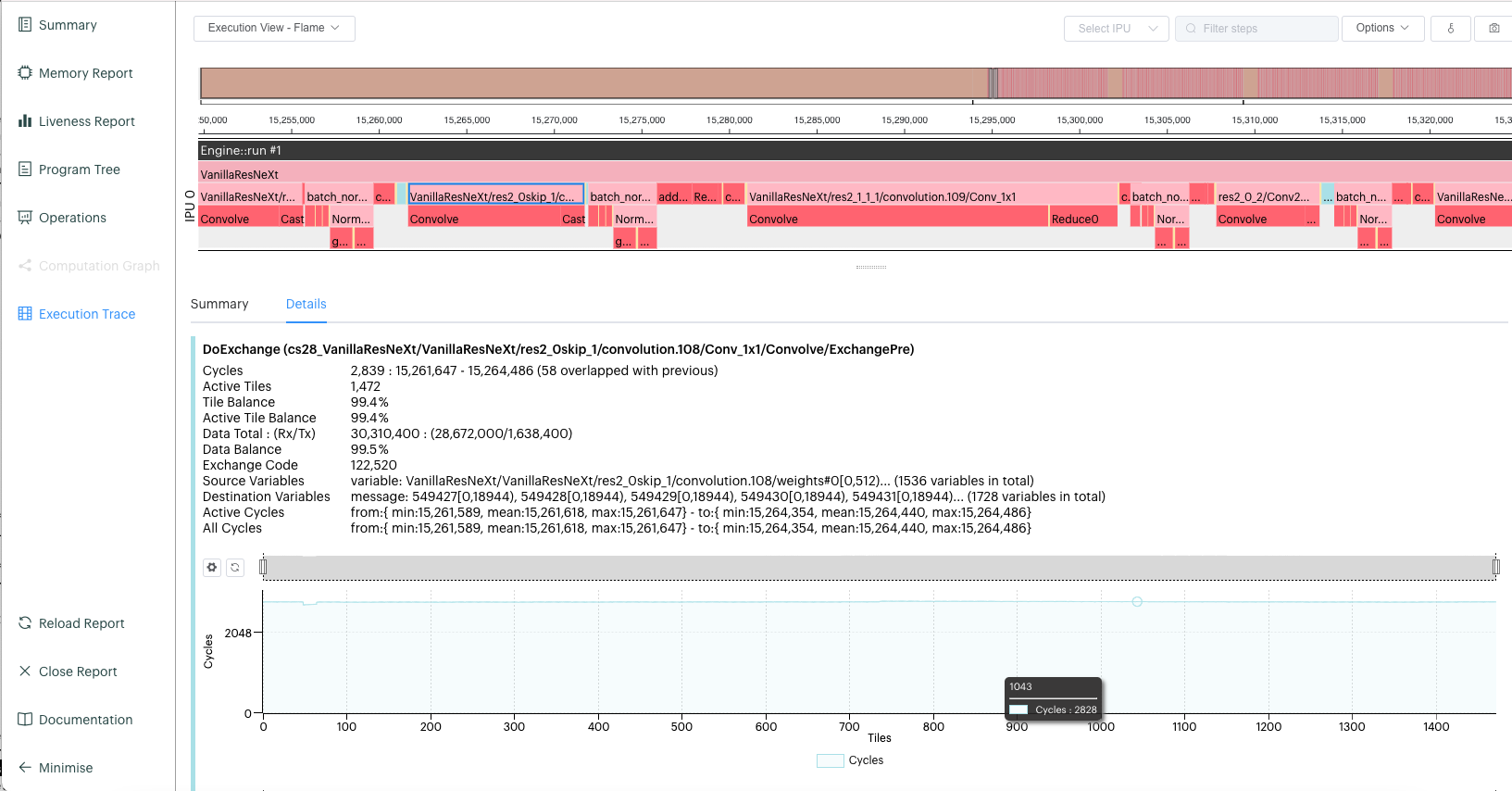
Two sample visualisations from the PopVision Graph Analyser are shown below.

Fig. 3.2 Cycle breakdown of inference pipeline. The beginning section is waiting time for the pre-processing. The orange section is the data transfer. Both can be decreased using infeeds and outfeeds as described in Section 3.5, Infeeds and outfeeds.

Fig. 3.3 Total memory usage of the IPU over processing time. The constant offset memory comes from the control code. The spikes in live-memory are characteristic of convolution or fully connected layers.

3.5. Infeeds and outfeeds

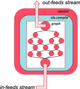
Infeeds and outfeeds are framework constructs that allow data to be streamed directly into and out ofa TensorFlow session. This creates a significant boost in data throughput since the host-to-device transfer is an active stack making data available as required. The concept is illustrated below.

Fig. 3.4 The infeeds/outfeeds construction in relation to a session

The Targeting the IPU from TensorFlow guide provides a description of data feeds. Here, we mainly summarize the data feeds construction in the sample script.

The first step is to create a dataset (lines 8 to 18) where the input data (in this case a synthetic tensor of [batch size, h, w, channels] dimension), is packaged into the dataset ds. Lines 66 to 71 instantiate the infeed and outfeed queues.

Within the network definition, three additions are required. Firstly, on line 44, a body(features) wrapper is defined to hold the model definition. Secondly, the output of the model is fed into the outfeed construct on line 49. Finally, the return statement of the model definition is a call to ipu.loops.repeat on line 50. On line 86, an outfeed dequeue is instantiated, which is the final preamble before a session definition. Within the session scope, an infeed queue is initialized on line 92, and after the session.run call to the compiled graph, the outfeed is dequeued. Data transfer thus follows a sequence of data upload into the infeed queue; session run of graph; data return via the outfeed queue.

Further aspects of this are presented within the guide and should be reviewed for greater insight.