1. Import the TensorFlow IPU module
First, we import the TensorFlow IPU module.
Add the import statement in Listing 1.1 to the beginning of your script.
from tensorflow.python import ipu
For the ipu module to function properly, we must import it directly
rather than accessing it through the top-level TensorFlow module.
2. IPU Config
To use the IPU, you must create an IPU session configuration in the main process. A minimum configuration is in Listing 2.1.
ipu_config = ipu.config.IPUConfig()
ipu_config.auto_select_ipus = 1  # Select 1 IPU for the model
ipu_config.configure_ipu_system()
This is all we need to get a small model up and running. A full list of configuration options is available in the Python API documentation.
3. Model
3.1. Single IPU models
You can train, evaluate or run inference on single-IPU models through
the Keras APIs as you would with other accelerators, as long as you
create the model inside the scope of an IPUStrategy. To do that,
first specify the IPU strategy and then wrap the model within the scope
of the IPU strategy.
3.1.1. Specify IPU strategy
tf.distribute.Strategy
is an API to distribute training across multiple devices. IPUStrategyV1
is a subclass which targets a system with one or more
IPUs attached. Another subclass, PopDistStrategy, targets a multi-system configuration.
To specify the IPU strategy, add the code in Listing 3.1 after the configuration.
# Create an execution strategy.
strategy = ipu.ipu_strategy.IPUStrategy()
3.1.2. Wrap the model within the IPU strategy scope
Creating variables and Keras models within the scope of the
IPUStrategy object will ensure that they are placed on the IPU. To
do this, we create a strategy.scope() context manager and move the
model code inside it as, for example, shown in Listing 3.2.
with strategy.scope():
    # Note model_fn() must return a dictionary with keys
    # `inputs` and `outputs`.
    model = keras.Model(*model_fn())

    # Compile our model with Stochastic Gradient Descent as an optimizer
    # and Categorical Cross Entropy as a loss.
    model.compile('sgd', 'categorical_crossentropy', metrics=["accuracy"])

    model.summary()
    print('\nTraining')
    model.fit(x_train, y_train, epochs=3, batch_size=64)
    print('\nEvaluation')
    model.evaluate(x_test, y_test)
Note that the function model_fn() defined by yourself can be readily reused.
All that is needed is to move the call to the function inside the context of
strategy.scope().
While all computation will now be performed on the IPU, the initialisation of variables will still be performed on the host.
3.2. Model parallelism
The models described so far occupy a single IPU device, however some models might require the model layers to be split across multiple IPU devices to achieve high compute efficiency.
One method to achieve model parallelism is called pipelining, where the model layers are assigned to pipeline stages. Each pipeline stage can be assigned to a different device and different devices can execute in parallel. There are three pipeline schedules: grouped (Fig. 3.1), interleaved (Fig. 3.2) and sequential (Fig. 3.3).
In the grouped schedule, the forward and backward stages are grouped together on each IPU. All IPUs alternate between executing a forward pass and then a backward pass. In the interleaved schedule, each pipeline stage executes a combination of forward and backward passes and in the sequential schedule, only one mini-batch is processed at a time.
Training performance depends on the chosen pipelining schedule. More information about the performance tradeoffs of pipelining can be found in the documentation Model parallelism with TensorFlow: sharding and pipelining.
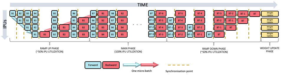
Fig. 3.1 Grouped pipeline schedule
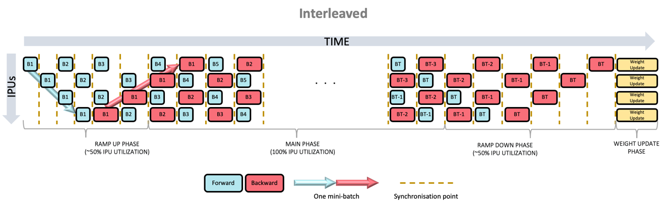
Fig. 3.2 Interleaved pipeline schedule
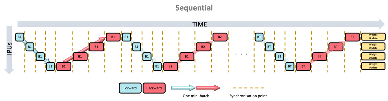
Fig. 3.3 Sequential pipeline schedule
The method to pipeline your model depends on whether your model is a
Sequential or a Functional model.
3.2.1. Sequential model
To enable IPU pipelining for a Sequential model (an instance of
tensorflow.keras.Sequential), a list of per-layer pipeline stage
assignments should be passed to the
set_pipeline_stage_assignment()
method of the model.
For example, a simple four-layer Sequential model could be assigned
to two different pipeline stages as in Listing 3.3.
model = tf.keras.Sequential([
      tf.keras.layers.Dense(8),  # Pipeline stage 0.
      tf.keras.layers.Dense(16),  # Pipeline stage 0.
      tf.keras.layers.Dense(16),  # Pipeline stage 1.
      tf.keras.layers.Dense(1),  # Pipeline stage 1.
  ])

  model.set_pipeline_stage_assignment([0, 0, 1, 1])
You can confirm which layers are assigned to which stages using the print_pipeline_stage_assignment_summary() method of the model.
3.2.2. Functional model
There are two ways to enable IPU pipelining for a Functional model
(an instance of tensorflow.keras.Model) depending on whether you’re
pipelining a model you are writing or an existing model.
Pipelining a model you are writing
To pipeline a Functional model you are writing yourself, each layer
call must happen within the scope of an ipu.keras.PipelineStage
context.
For example, a simple four-layer Functional model could be assigned
to two different pipeline stages as in Listing 3.4.
 input_layer = tf.keras.layers.Input((28, 28))

  with ipu.keras.PipelineStage(0):
    x = tf.keras.layers.Dense(8)(input_layer)
    x = tf.keras.layers.Dense(16)(x)

  with ipu.keras.PipelineStage(1):
    x = tf.keras.layers.Dense(16)(x)
    x = tf.keras.layers.Dense(1)(x)

  model = tf.keras.Model(inputs=input_layer, outputs=x)
Pipelining an existing functional model
To pipeline an existing Functional model, you can use
get_pipeline_stage_assignment().
Each layer invocation in the model has an associated
FunctionalLayerPipelineStageAssignment
object, which indicates which pipeline stage that invocation is assigned
to. get_pipeline_stage_assignment returns a list of these stage
assignments, which you can inspect and modify. Note that the list is in
post-order, which means the assignments are returned in the order they
will be executed.
Once you are done modifying the stage assignments, you should use set_pipeline_stage_assignment() to set them on the model.
For example, a naive way of pipelining ResNet50 would be to assign
everything up until the conv4_block2_add layer invocation to the first
stage, then everything else to the second stage, as in Listing 3.5.
strategy = ipu.ipu_strategy.IPUStrategy()
with strategy.scope():

  from tensorflow.keras.applications.resnet50 import ResNet50
  model = ResNet50(weights='imagenet')

  # Get the individual assignments - note that they are returned in post-order.
  assignments = model.get_pipeline_stage_assignment()

  # Iterate over them and set their pipeline stages.
  stage_id = 0
  for assignment in assignments:
    assignment.pipeline_stage = stage_id
    # Split the model on the `conv4_block2_add` layer.
    if assignment.layer.name.startswith("conv4_block2_add"):
      stage_id = 1

  # Set the assignments to the model.
  model.set_pipeline_stage_assignment(assignments)
    # print the pipeline stage assignments of the model’s layer invocations.
  model.print_pipeline_stage_assignment_summary()
4. Training process
4.1. Using model.fit
The example in this section (Listing 4.1) highlights the use of model.fit for the training process.
import tensorflow as tf
from tensorflow.python import ipu

# Configure the IPU device.
config = ipu.config.IPUConfig()
config.auto_select_ipus = 1
config.configure_ipu_system()


# Create a simple model.
def create_model():
  return tf.keras.Sequential([
      tf.keras.layers.Flatten(),
      tf.keras.layers.Dense(256, activation='relu'),
      tf.keras.layers.Dense(128, activation='relu'),
      tf.keras.layers.Dense(10)
  ])


# Create a dataset for the model.
def create_dataset():
  mnist = tf.keras.datasets.mnist

  (x_train, y_train), (_, _) = mnist.load_data()
  x_train = x_train / 255.0

  train_ds = tf.data.Dataset.from_tensor_slices(
      (x_train, y_train)).shuffle(10000).batch(32, drop_remainder=True)
  train_ds = train_ds.map(lambda d, l:
                          (tf.cast(d, tf.float32), tf.cast(l, tf.int32)))

  return train_ds.repeat().prefetch(16)

dataset = create_dataset()

# Create a strategy for execution on the IPU.
strategy = ipu.ipu_strategy.IPUStrategy()
with strategy.scope():
  # Create a Keras model inside the strategy.
  model = create_model()

  # Compile the model for training.
  model.compile(
      loss=tf.keras.losses.SparseCategoricalCrossentropy(),
      optimizer=tf.keras.optimizers.RMSprop(),
      metrics=["accuracy"],
      steps_per_execution=50,
  )

  model.set_gradient_accumulation_options(

      gradient_accumulation_steps_per_replica=10)

  model.fit(dataset, epochs=2, steps_per_epoch=100)
4.2. Customized training loop
4.2.1. Training loops, data sets and feed queues
To construct a system that will train in a loop, you will need to do the following:
Wrap your optimiser training operation in a loop.
Create a TensorFlow dataset to provide data to the input queue. Note the datasets iterator must be created outside the strategy scope, unless the flag
enable_dataset_iteratorsofIPUStrategyV1()is set toFalse.
The following example (Listing 4.2) shows how to construct a trivial TensorFlow dataset (tf.data.Dataset), attach it to a model using an IPUInfeedQueue, feed results into an IPUOutfeedQueue, and construct a loop.
from tensorflow.python.ipu import ipu_infeed_queue
from tensorflow.python.ipu import ipu_outfeed_queue
from tensorflow.python.ipu import loops
from tensorflow.python.ipu import ipu_strategy
from tensorflow.python.ipu.config import IPUConfig
import tensorflow as tf

# The dataset for feeding the graphs
ds = tf.data.Dataset.from_tensors(tf.constant(1.0, shape=[800]))
ds = ds.map(lambda x: [x, x])
ds = ds.repeat()

# The host side queues
outfeed_queue = ipu_outfeed_queue.IPUOutfeedQueue()

# The device side main
def body(x1, x2):
   d1 = x1 + x2
   d2 = x1 - x2
   return {'d1': d1, 'd2': d2}

@tf.function(experimental_compile=True)
def my_net(dataset_iterator, outfeed_queue):
   for _ in tf.range(10):
      d1, d2 = next(dataset_iterator)
      outfeed_queue.enqueue(body(d1, d2))

# Configure the IPU system.
config = IPUConfig()
config.auto_select_ipus = 1
config.configure_ipu_system()

# Initialize the IPU default strategy.
strategy = ipu_strategy.IPUStrategyV1()

with strategy.scope():
   # Create an iterator on the dataset
   dataset_iterator = iter(ds)

   # Run the graph on the IPU.
   strategy.run(my_net, args=[dataset_iterator, outfeed_queue])

   # The outfeed dequeue has to happen after the outfeed enqueue op has been executed.
   result = outfeed_queue.dequeue()

   print("outfeed result", result)
In this case, the dataset is a trivial one. It constructs a tf.data.Dataset from a single TensorFlow constant, and then maps the output of that dataset into a pair of tensors. It then arranges for the dataset to be
repeated indefinitely.
After the dataset is constructed, the output data feed queue is constructed. An
infeed queue is not required since TensorFlow 2.4 supports using dataset
iterators as infeed an queue. The IPUOutfeedQueue has extra options to
control how it collects and outputs the data sent to it. None of these are used
in
Listing 4.2.
Now that we have tf.data.Dataset and the queues for getting data in and out
of the device-side code, we can construct the device-side part of the
model. In this example, the body function constructs a very simple
model, which does not even have an optimiser. It takes the two data
samples which will be provided by the dataset, and performs some simple
maths on them, and inserts the results into the output queue.
Typically, in this function, the full machine learning model would be constructed and a TensorFlow Optimizer would be used to generate a backward pass and variable update operations. The returned data would typically be a loss
value. If we are only calling the training operation, then no data is returned.
The my_net function wraps the body function in a loop. Since the loop is
created inside a @tf.function, the loop will be compiled to run on the device.
Data will be fed from the host via the implicit infeed queue created by the
dataset’s iterator. The results of the program on the IPU device will be sent to
the hosts via the explicit outfeed queue outfeed_queue.
Next, we create an IPU scope at the top level and call strategy.run
passing the my_net function, to create the training loop in the main
graph. Finally, we create an operation which can be used to fetch
results from the outfeed queue. Note that it isn’t necessary to use an
outfeed queue if you do not wish to receive per-sample output from the
training loop. If all you require is the final value of a tensor, then
it can be output normally without the need for a queue.
If you run the example, then you will find that the result is a Python dictionary containing two numpy arrays. The first is the d1 array
and will contain x1 + x2 for each iteration in the loop. The second
is the d2 array and will contain x1 - x2 for each iteration in
the loop.
For a more practical example, the Graphcore tutorials contain a detailed tutorial about using infeeds and outfeeds with TensorFlow.
4.2.2. Accessing outfeed queue results during execution
An IPUOutfeedQueue supports the results being fetched continuously
during the execution of a model. This feature can be used to monitor the
performance of the network, for example to check that the loss is
decreasing, or to stream predictions for an inference model to achieve
minimal latency for each sample.
from threading import Thread

from tensorflow.python import ipu
import tensorflow as tf

NUM_ITERATIONS = 100

#
# Configure the IPU system
#
cfg = ipu.config.IPUConfig()
cfg.auto_select_ipus = 1
cfg.configure_ipu_system()


#
# The input data and labels
#
def create_dataset():
  mnist = tf.keras.datasets.mnist

  (x_train, y_train), (_, _) = mnist.load_data()
  x_train = x_train / 255.0

  train_ds = tf.data.Dataset.from_tensor_slices(
      (x_train, y_train)).shuffle(10000)
  train_ds = train_ds.map(lambda d, l:
                          (tf.cast(d, tf.float32), tf.cast(l, tf.int32)))
  train_ds = train_ds.batch(32, drop_remainder=True)
  return train_ds.repeat()


#
# The host side queue
#
outfeed_queue = ipu.ipu_outfeed_queue.IPUOutfeedQueue()


#
# A custom training loop
#
@tf.function(experimental_compile=True)
def training_step(num_iterations, iterator, in_model, optimizer):

  for _ in tf.range(num_iterations):
    features, labels = next(iterator)
    with tf.GradientTape() as tape:
      predictions = in_model(features, training=True)
      prediction_loss = tf.keras.losses.sparse_categorical_crossentropy(
          labels, predictions)
      loss = tf.reduce_mean(prediction_loss)
      grads = tape.gradient(loss, in_model.trainable_variables)
      optimizer.apply_gradients(zip(grads, in_model.trainable_variables))

    outfeed_queue.enqueue(loss)


#
# Execute the graph
#
strategy = ipu.ipu_strategy.IPUStrategyV1()
with strategy.scope():
  # Create the Keras model and optimizer.
  model = tf.keras.models.Sequential([
      tf.keras.layers.Flatten(),
      tf.keras.layers.Dense(128, activation='relu'),
      tf.keras.layers.Dense(10, activation='softmax')
  ])
  opt = tf.keras.optimizers.SGD(0.01)

  # Create an iterator for the dataset.
  train_iterator = iter(create_dataset())

  # Function to continuously dequeue the outfeed until NUM_ITERATIONS examples
  # are seen.
  def dequeue_thread_fn():
    counter = 0
    while counter != NUM_ITERATIONS:
      for loss in outfeed_queue:
        print("Step", counter, "loss = ", loss.numpy())
        counter += 1

  # Start the dequeuing thread.
  dequeue_thread = Thread(target=dequeue_thread_fn, args=[])
  dequeue_thread.start()

  # Run the custom training loop over the dataset.
  strategy.run(training_step,
               args=[NUM_ITERATIONS, train_iterator, model, opt])
  dequeue_thread.join()
5. Optimization
5.1. Memory optimization
5.1.1. IPU specific/optimized layers
Use IPU-optimized layers instead of the original TensorFlow versions. There are also many IPU-specific layers which can greatly utilize the performance of IPU. You can find all Keras layer specializations for the IPU in the IPU TensorFlow Addons.
5.1.2. Reduce available_memory_proportion
Change the value of the availableMemoryProportion parameter. This is the proportion of IPU memory that can be used as temporary memory by a convolution or matrix multiplication. The default proportion is set to 0.6, which aims to balance execution speed against memory. To fit larger models on the IPU, a good first step is to lower the available memory proportion to force the compiler to optimise for memory use over execution speed. Less temporary memory means more cycles to execute. It also increases always-live memory as more control code is needed to deal with the planning of the split calculations. Reducing this value too far can result in out-of-memory (OOM) errors . We recommend setting this to a value greater than 0.05.
For more information on using availableMemoryProportion for
optimising temporary memory use for convolutions and matrix multiplies
on the IPU, refer to the technical note Optimising Temporary Memory
Usage for Convolutions and Matmuls on the IPU
5.1.3. Enable Replicated Tensor Sharding
Replication is a form of data parallelism where the computational graph is replicated and run in parallel.
If a tensor in a replicated graph with replication factor R has the same value on each replica, you can save memory by storing just a fraction (1/R), called a shard, of the tensor on each replica. When the full tensor is required all R shards can be broadcast to all the replicas. This only applies when the tensor has the same value on every replica, for example the tensor containing the optimiser states.
Replicated tensor sharding is typically performed on the optimiser state variables. So, to enable replicated tensor sharding, you need to set replicated_optimizer_state_sharding in the Model.set_pipelining_options() function. For more information on setting pipelining options, see the
TensorFlow 2 API documentation.
5.1.4. Variable Offloading
When using pipelining to train a model, it is possible to offload certain variables into off-chip Streaming Memory. This feature can allow savings of In-Processor-Memory memory, at the cost of time spent communicating with the host when the offloaded variables are needed on the device. The API supports offloading of the weight update variables and activations.
The weight update variables are any tf.Variable only accessed and
modified during the weight update of the pipeline. An example is the
accumulator variable of tf.MomentumOptimizer. This means that
these variables do not need to be stored in device memory during the
forward and backward propagation of the model, so when
offload_weight_update_variables is enabled these variables are
streamed onto the device during the weight update and then streamed back
to Streaming Memory after they have been updated.
When offload_activations is enabled, all the activations for the
mini-batches which are not being executed by the pipeline stages at any
given time are stored in the Streaming Memory. So, in an analogous way
as described above, when an activation is needed for computation, it is
streamed onto the device, and then streamed back to the Streaming Memory
after it has been used.
For more information on variable offloading, see the TensorFlow 2 API documentation: Optimizer state offloading.
5.1.5. Recomputation
Tensors are stored in memory (referred to as “live”) for as long as they are required. By default, we need to store the activations from the forward pass until they are consumed during backpropagation. In the case of pipelining, tensors can be kept live for quite a long time. We can reduce this liveness, and therefore the memory requirements, by recomputing the activations.
Rather than storing all the activations within a pipeline stage, we retain only the activations that feed the input of the stage (called a “stash”). The other internal activations within the stage are calculated from the stashes just before they are needed in the backward pass for a given batch. The stash size is equivalent to the number of pipeline stages, as that reflects the number of batches being processed in parallel. Hence as you increase the number of stages in a pipeline, the stash overhead also increases accordingly.
Recomputation can be enabled by setting
allow_recompute
in IPUConfig. Enabling this option can reduce memory usage at the
expense of extra computation. For smaller models, it can allow us to
increase batch-size and therefore efficiency.
A demonstration of pipeline recomputation can be found in the technical note Model parallelism with TensorFlow: sharding and pipelining.
5.2. Throughput
5.2.1. Using steps_per_execution
The IPU implementation above is fast, but not as fast as it could be. This is because, unless we specify otherwise, the program that runs on the IPU will only process a single batch, so we cannot improve performance from loading the data asynchronously and using a looped version of this program.
To change this, we must set the steps_per_execution argument in
model.compile(). This sets the number of batches processed in each
execution of the underlying IPU program. Make a copy of
completed_demos/completed_demo_ipu.py, and change the code for
adjusting the lengths of the datasets as in Listing 5.1.
# Adjust dataset lengths to be divisible by the batch size
train_data_len = x_train.shape[0]
train_steps_per_execution = train_data_len // batch_size
train_data_len = make_divisible(train_data_len, train_steps_per_execution * batch_size)
x_train, y_train = x_train[:train_data_len], y_train[:train_data_len]

test_data_len = x_test.shape[0]
test_steps_per_execution = test_data_len // batch_size
test_data_len = make_divisible(test_data_len, test_steps_per_execution * batch_size)
x_test, y_test = x_test[:test_data_len], y_test[:test_data_len]
The number of examples in the dataset must be divisible by the number of
examples processed per execution (that is,
steps_per_execution * batch_size). Here, we set
steps_per_execution to be (length of dataset) // batch_size for
maximum throughput and so that we do not lose any more data than we
must, though this code should work just as well with a smaller value.
Now we update the code from with strategy.scope(): onwards by
passing steps_per_execution as an argument to model.compile(),
and providing our batch_size value to model.fit() and
model.evaluate(). We can re-compile the model with a different value
of steps_per_execution between running model.fit() and
model.evaluate(), so we do so here, although it isn’t compulsory.
with strategy.scope():
    model = keras.Model(*model_fn())

    # Compile our model with Stochastic Gradient Descent as an optimizer
    # and Categorical Cross Entropy as a loss.
    model.compile('sgd', 'categorical_crossentropy',
                  metrics=["accuracy"],
                  steps_per_execution=train_steps_per_execution)
    model.summary()
    print('\nTraining')
    model.fit(x_train, y_train, epochs=3, batch_size=batch_size)
    model.compile('sgd', 'categorical_crossentropy',
                  metrics=["accuracy"],
                  steps_per_execution=test_steps_per_execution)
    print('\nEvaluation')
    model.evaluate(x_test, y_test, batch_size=batch_size)
5.2.2. Replication
Another way to speed up the training of a model is to make a copy of the model on each of multiple IPUs, updating the parameters of the model on all IPUs after each forward and backward pass. This is called replication and can be done in Keras with very few code changes.
First, in the main process or in the data loader process, we’ll add variables for the number of IPUs and the number of replicas as in Listing 5.3.
# Variables for model hyperparameters
num_classes = 10
input_shape = (28, 28, 1)
batch_size = 64
num_ipus = num_replicas = 2
Because our model is written for one IPU, the number of replicas will be equal to the number of IPUs.
We will need to adjust for the fact that with replication, a batch is
processed on each replica for each step, so steps_per_execution
needs to be divisible by the number of replicas. Also, the maximum value
of steps_per_execution is now
train_data_len // (batch_size * num_replicas), since the number of
examples processed in each step is now (batch_size * num_replicas).
We therefore add two lines to the dataset-adjustment code as in Listing 5.4.
def make_divisible(number, divisor):
    return number - number % divisor

# Adjust dataset lengths to be divisible by the batch size
train_data_len = x_train.shape[0]
train_steps_per_execution = train_data_len // (batch_size * num_replicas)
# `steps_per_execution` needs to be divisible by the number of replicas
train_steps_per_execution = make_divisible(train_steps_per_execution, num_replicas)
train_data_len = make_divisible(train_data_len, train_steps_per_execution * batch_size)
x_train, y_train = x_train[:train_data_len], y_train[:train_data_len]

test_data_len = x_test.shape[0]
test_steps_per_execution = test_data_len // (batch_size * num_replicas)
# `steps_per_execution` needs to be divisible by the number of replicas
test_steps_per_execution = make_divisible(test_steps_per_execution, num_replicas)
test_data_len = make_divisible(test_data_len, test_steps_per_execution * batch_size)
x_test, y_test = x_test[:test_data_len], y_test[:test_data_len]
We’ll need to acquire multiple IPUs, so we update the configuration step as in Listing 5.5.
ipu_config = ipu.config.IPUConfig()
ipu_config.auto_select_ipus = num_ipus
ipu_config.configure_ipu_system()
These are all the changes we need to make to replicate the model and
train on multiple IPUs. There is no need to explicitly copy the model or
organise the exchange of weight updates between the IPUs because all
these details are handled automatically, as long as we select multiple
IPUs and create and use our model within the scope of an IPUStrategy
object.
5.2.3. Increase the gradient accumulation count
The larger the gradient accumulation count:
The smaller the proportion of time spent during a weight update.
The smaller the proportion of time spent during ramp up and ramp down.
An increase in gradient accumulation count yields these reductions by performing the forward and backward passes on a greater number of mini-batches prior to the updating of weights and parameters. This results in a larger global batch size. The computed gradients for each mini-batch are aggregated, for example by reduction to the mean or sum, such that the weight update is performed with the larger, aggregated batch.
In Fig. 5.1, the processing of four mini-batches is shown without gradient accumulation. It can be seen that immediately following the forward and backward passes of each mini-batch is a weight update stage.
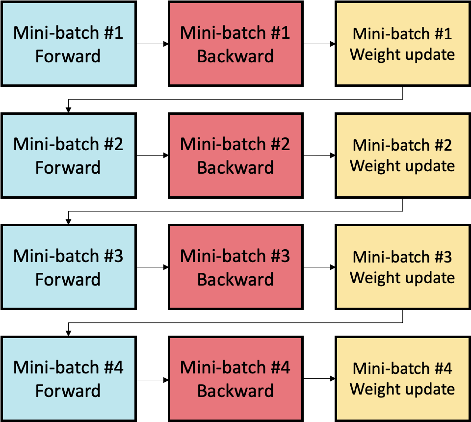
Fig. 5.1 Not using gradient accumulation
However, when processing the four-mini batches of Fig. 5.1 with a gradient accumulation count of four, it can be seen in Fig. 5.2 that only a single weight update stage is performed. This is due to the aggregation of the gradients computed in the backward pass for each mini-batch.
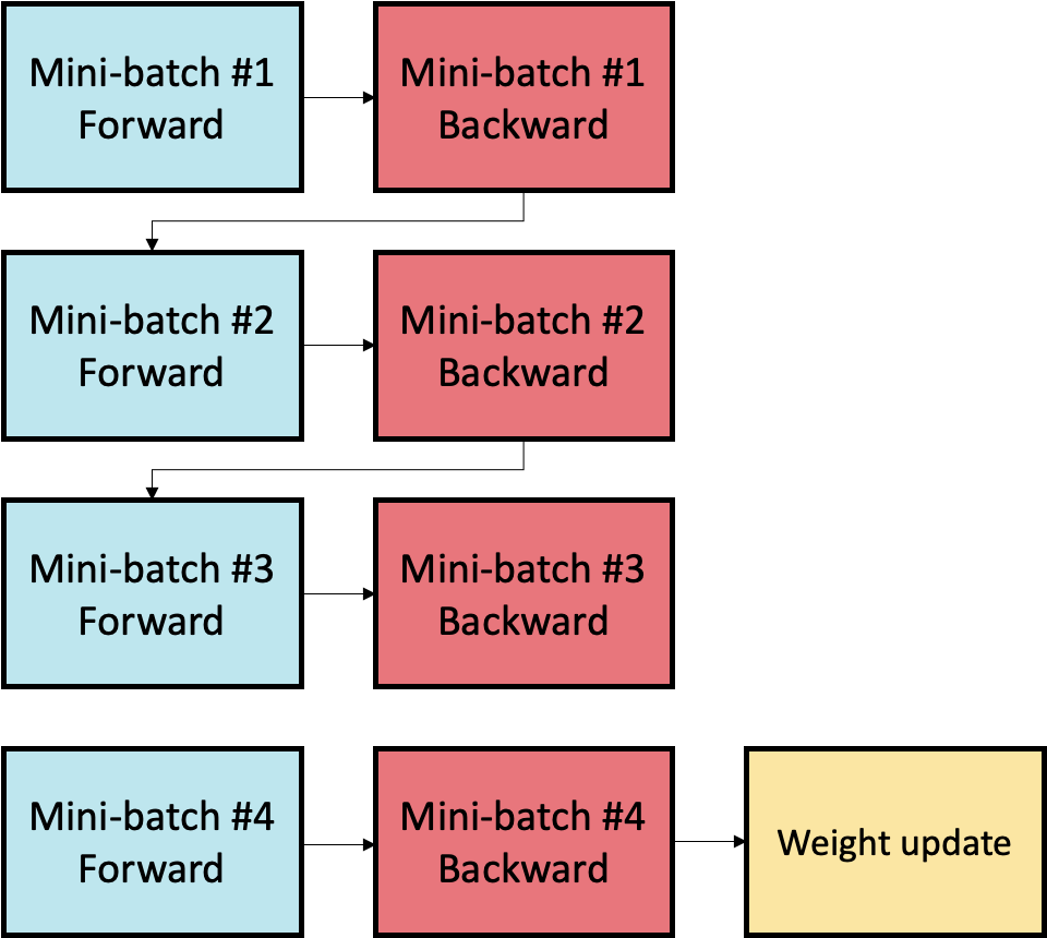
Fig. 5.2 Using a gradient accumulation count of 4
As weight updates are performed following the ramp down phase of pipeline execution, the use of a higher gradient accumulation count will also reduce the number of ramp up/ramp down cycles between batches as the effective batch size will be larger, as previously outlined. As ramp up and ramp down fill and clear the pipeline, reducing occurrences of ramp up and ramp down maximises time spent on compute. A lower gradient accumulation count will incur more ramp up/ramp down cycles, causing more time to be spent filling and clearing the pipeline.