3. Programming model
This section describes the IPU abstract programming model, as well as techniques for compiling and running IPU programs.
3.1. The Poplar graph libary
The programming model described in this section is implemented in the Poplar
graph library (libpoplar). This library provides an API for constructing and
running IPU programs and performs the necessary compilation to run the programs
on IPU devices. Refer to the Poplar and PopLibs User Guide for more information.
3.2. Programs
Programs run over a set of IPUs. This set is user configurable and is chosen before the program is compiled. The set of IPUs running a program does not change over the course of the program’s execution.
A single program runs across all the selected IPUs. This program will follow a path of specified control flow and manipulate variables just like a standard program for a CPU. The variables being manipulated are large arrays of data (which are often interpreted as multi-dimensional tensors) that live across the various memory elements of the IPUs and Streaming Memory. The program manipulates these variables with a set of highly parallel tasks (called vertices) executed on the threads of the tile processors. These sets of tasks are known as compute sets. Fig. 3.1 shows the overall structure of programs on the IPU.
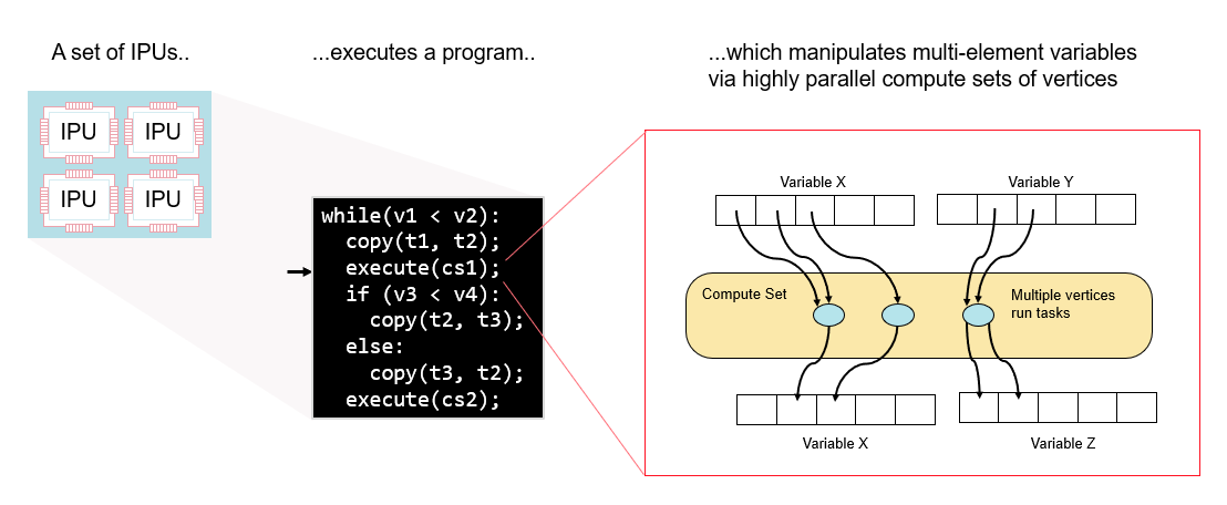
Fig. 3.1 Programs running on a set of IPUs
Note that even though the program runs across all IPUs, the IPU is not a SIMD device. There is not a single machine-level instruction stream that is distributed to the IPUs. Instead, the IPUs synchronise at known points to run the program. This allows the flexibility for completely different code to run on every parallel thread between synchronisation points.
3.2.1. Data variables
Variables hold data whilst a program is executed. On each set of tiles, the programs manipulate typed arrays (of fixed size). For example, a variable could be an array containing 1024 elements of type float (32 bit floating-point numbers).
A single variable may be stored across the memory units of multiple tiles. Each element of the variable is placed on or “mapped” to a specific tile. This is called the tile mapping of the variable.
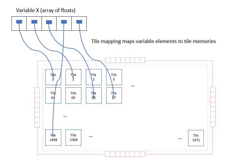
Fig. 3.2 A variable and its mapping to tiles
Variables always have global scope. They can be read or written at any part of the program, but the physical memory allocated for a variable might be shared with other variables that are not needed at the same time (Section 3.5.1, Variable liveness).
When ML programs manipulate variables, it is often useful to view them as multi-dimensional tensors. In this case, different parts of the program may want to view the base variable as a different kind of tensor (for example, viewing a matrix as either row-major or column-major). So, for programs on the IPU, a tensor is a view onto an underlying variable.
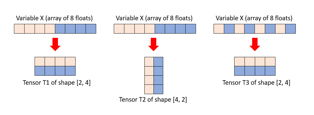
Fig. 3.3 Multiple views on the same variable
Looking at variables as multi-dimensional tensors is extremely useful for building the access patterns needed to run programs on the IPU. However, the data manipulation still happens on the underlying variable in memory.
Variables can be stored across the tiles and in Streaming Memory (Section 2.1, Memory architecture).
The Poplar graph library provides a rich set of operators for creating tensor views of variables including slicing, transposition and concatenation to build up tensors. Refer to the Poplar Tensor API for details.
3.2.2. Copying data and executing compute sets
As a program executes on a tile set it will manipulate the variables in the program. There are two main ways of doing this: copying data and executing compute sets.
The most basic copying involves just copying one variable to another, for example:
Copy(v1, v2);
However, copying can also include rearrangements of fixed patterns. This can be done via the tensor views described in Section 3.2.1, Data variables. For example, copying from a transposed view will perform a transpose copy:
Copy(t1.tranpose(), t2);
Here, t1.transpose() just provides a view of the rearranged data elements but by using it as the source of the copy operation to a new variable, it will actually perform the rearrangement and will move the data in memory.
Compute sets execute code to manipulate data. Each compute set has a name:
Execute(cs1)
When a compute set runs, it reads, computes and writes a set of variable elements from the variables of the program:
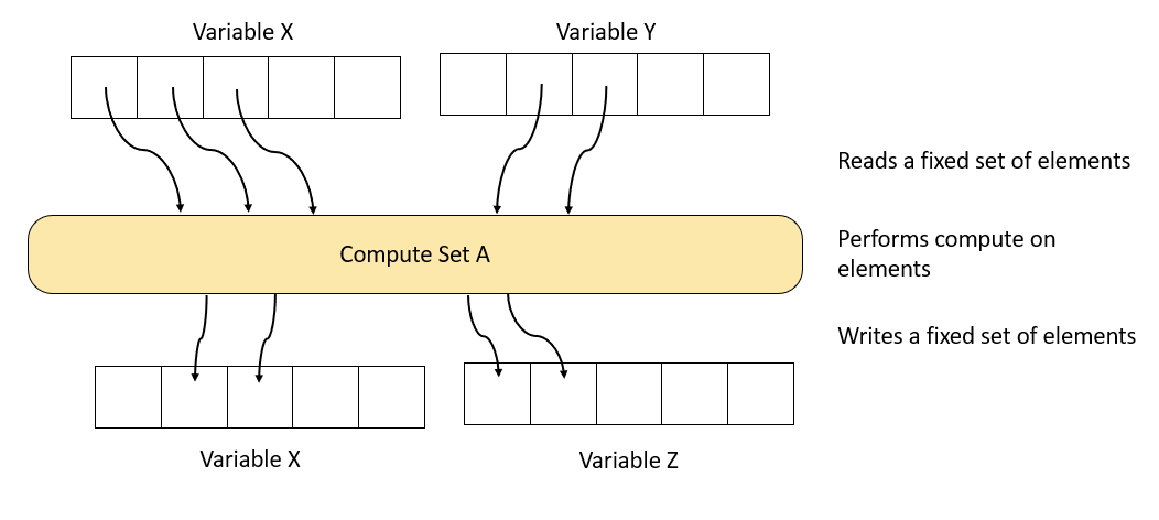
Fig. 3.4 A compute set
Note
The variable elements that are accessed by any particular compute set are fixed — they cannot vary on each execution.
A compute set may perform many different computations, for example incrementing every element of a variable. How the program specifies what function the compute set executes is described in Section 3.2.4, Compute sets.
3.2.3. Control flow: sequences, conditionals and loops
In addition to the basic operations of copying data and executing compute sets, programs running on the IPU can execute standard control flow: loops, conditionals etc. For example:
while(v1 < v2):
  copy(t1, t2);
  execute(cs1);
  if (v3 < v4):
    copy(t2, t3);
  else:
    copy(t3, t2);
  execute(cs2);
Here the variables used for control flow are tensors of size 1 (that is, scalars) mapped to standard variables (for example, v1 in
Listing 3.1) that can be manipulated by compute sets.
The overall control flow defined by the program is the same for all tiles on all IPUs. Conceptually, there is a single program which defines the global control flow applied to all the IPUs in the system. Note however, that this global program is decoupled from the computation performed by each vertex in the graph (as explained at the beginning of the chapter, the machine is not SIMD, every vertex can be running an independent program). Each tile can take a different path through the program. It will decide which branch of a conditional to execute, or how many iterations of a loop to execute, depending on its local data.
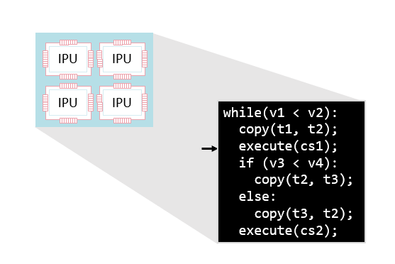
Fig. 3.5 The entire system of IPUs runs a single program
3.2.4. Compute sets
A compute set is a highly parallel piece of compute. Each compute set consists of many vertices that are compute tasks. Each vertex within the compute set executes a piece of code in parallel to the other vertices. So, in Fig. 3.4, the compute set that performs computation and reads and writes variables is actually a set of vertices running in parallel, each one of which reads and writes variables and performs computation.
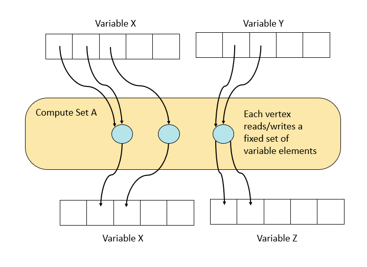
Fig. 3.6 The vertices within a compute set
The vertices determine how a compute set splits its tasks into fine-grained, parallel pieces of compute to use the many tiles and worker threads on the IPU. Each vertex is tied to a specific tile of the IPU.
Each vertex runs a small piece of code (separate to the main program) that processes its own input and output. The piece of code that a vertex runs is known as a codelet. The combination of each vertex running this code in parallel is what defines the function of the compute set. More information on programming vertices can be found in the Poplar and PopLibs User Guide.
3.2.5. The computational graph
The vertices from the multiple compute sets in a program form the computational graph of the program as in Fig. 3.7.
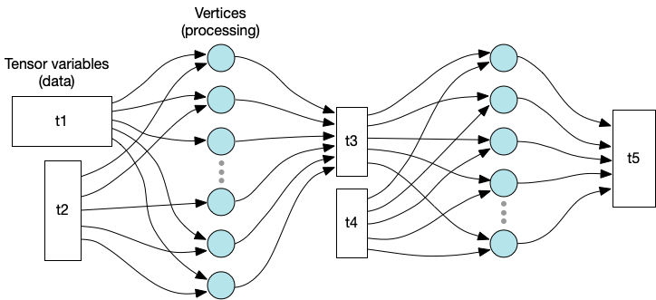
Fig. 3.7 Graph representation of variables and processing
This graph holds the relationship between compute and data which is explicit and created with the program. The graph shows the data relationships but not the control flow of the program.
3.2.6. Data streams
Programs running on the IPU have access to connections to external data. These data streams allow the program to copy data from an external source (usually the memory of a host computer) into a variable of a program.
..
stream-copy(s1, v1)
execute(cs)
copy(v1, v2)
The configuration of how data is provided or consumed from data streams is configured by the host when the program is executed (see Section 3.3, Loading and running programs).
Since data stream copies generally go through multiple memories (host memory and Streaming Memory) before getting to the IPU, there are several implementation-specific flags to optimise the transfer (for example, enabling overlap of the memory transfers by prefetching data). Details of these options can be found in the Poplar and PopLibs User Guide and a practical discussion of how these optimisations can apply to an application can be found in The Memory and Performance Optimisation Guide.
3.2.7. IPU-level task parallelism
As well as the fine-grained parallelism at each compute set, the program running on a set of IPUs can also be split into parallel sub-programs via fork-join style parallelism.
Since all tiles within an IPU are grouped together for synchronisation, the parallelisation of the program works at a granularity where the individual sub-programs run on different IPUs. Fig. 3.8 shows this.
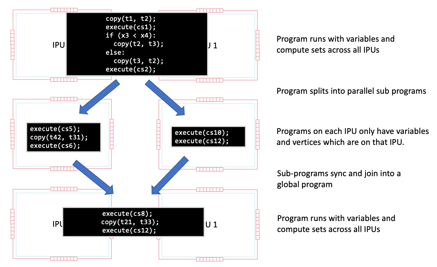
Fig. 3.8 A program splitting into parallel sub-programs
This capability is used for several programming techniques, such as pipeline model parallelism, and is described in Section 5, Common algorithmic techniques for IPUs.
3.2.7.1. Overlapping I/O within the IPU
In addition to the general method of running programs in parallel on different IPUs, a limited form of task parallelism can be executed within the IPU. The IPU can be split into two sets of tile groups. One tile group only performs I/O to fetch and receive data from outside of the chip and the other tile group can perform general compute. The program is then split into two sub-programs to run in parallel with one of the sub-programs just running a sequence of either data stream or copies to and from variables held in Streaming Memory onto the tile group dedicated to I/O.
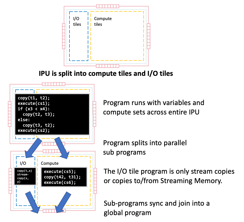
Fig. 3.9 Parallel execution of I/O
3.3. Loading and running programs
A multi-IPU device will always be connected to a host which controls the compilation and execution of programs.
First, the host will construct a set of programs to run on a set of IPUs. These programs are then compiled together into a binary which is then loaded onto the IPUs.
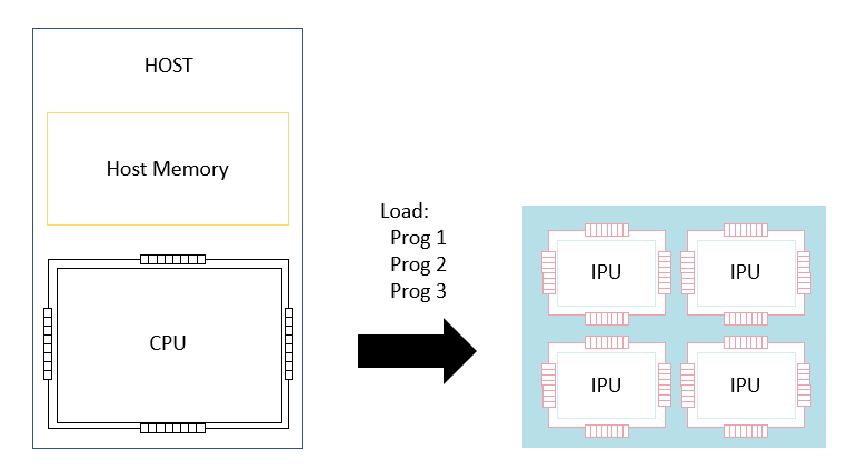
Fig. 3.10 Loading programs on to the IPU
In addition to loading the programs, the host needs to configure what happens when a program reads from or writes to one of its data streams. This is done up-front by the host application which will either connect a datastream to a data source (for example, a region of host memory) or to a handler on the host which will deal with data stream requests from the IPU.
Once the programs are loaded and configured, the host can then instruct the IPUs to run one of the programs.
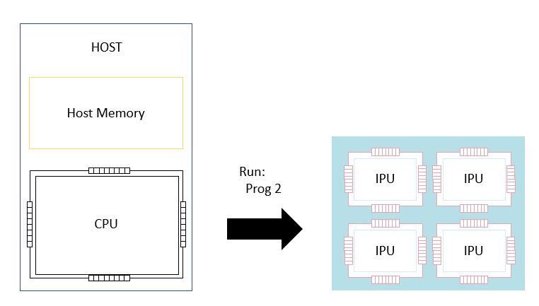
Fig. 3.11 Selecting a control program to run
At this point the IPUs will execute the entire selected program. During this program’s execution, the IPUs can read and write data from data streams. For example, the program can issue instructions to pull items of training data onto the IPU when training a neural network model (the model itself is already resident on the processor).
3.4. The implementation of ML frameworks using IPU programs
Higher-level machine-learning frameworks such as PyTorch and TensorFlow let you specify computational graphs that provide models of external phenomena. These graphs have learnable parameters which the frameworks can then train with an optimisation algorithm specified in the framework that consumes training data.
The implementation flow from a typical high-level framework to an IPU program is shown in Fig. 3.12.
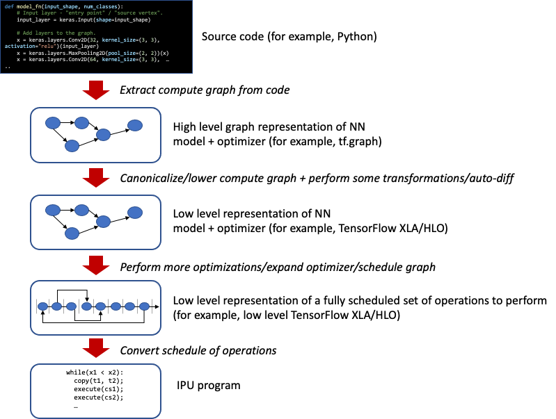
Fig. 3.12 A typical framework lowering to run on an IPU
The framework will perform transformations on the computational graph, add the backward passes and optimiser loops to that graph and finally schedule the graph such that each node is computed in a particular order. Once a scheduled graph is in place, it can be translated into an IPU program where each node is replaced by the execution of compute sets.
3.5. The compilation and execution of IPU programs
The program executed on an IPU is conceptually executed across all the IPUs together. However, the IPUs have completely disjoint memories (Fig. 2.3) and so do not have direct access to a shared state.
This means that the program cannot be passed through a conventional compiler to execute on the set of tiles. Instead the program is first lowered into a form that matches IPU chip execution (consisting of sync, exchange and compute as described in Section 2.2, Execution).
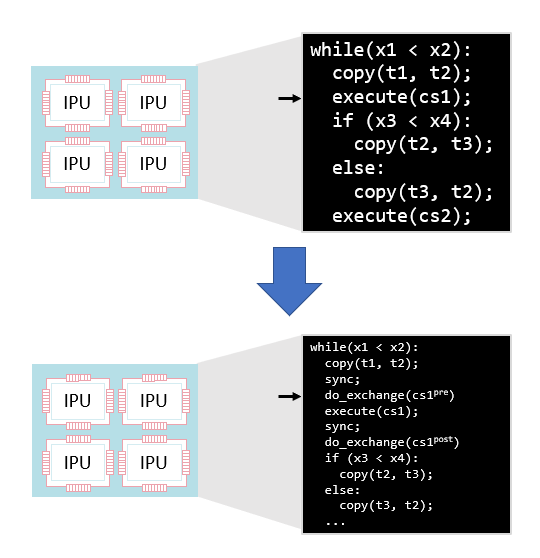
Fig. 3.13 Lowering a program to explicit sync, exchange and compute steps
The global program is then lowered to a program for each tile with explicit synchronisation and communication steps on each tile.
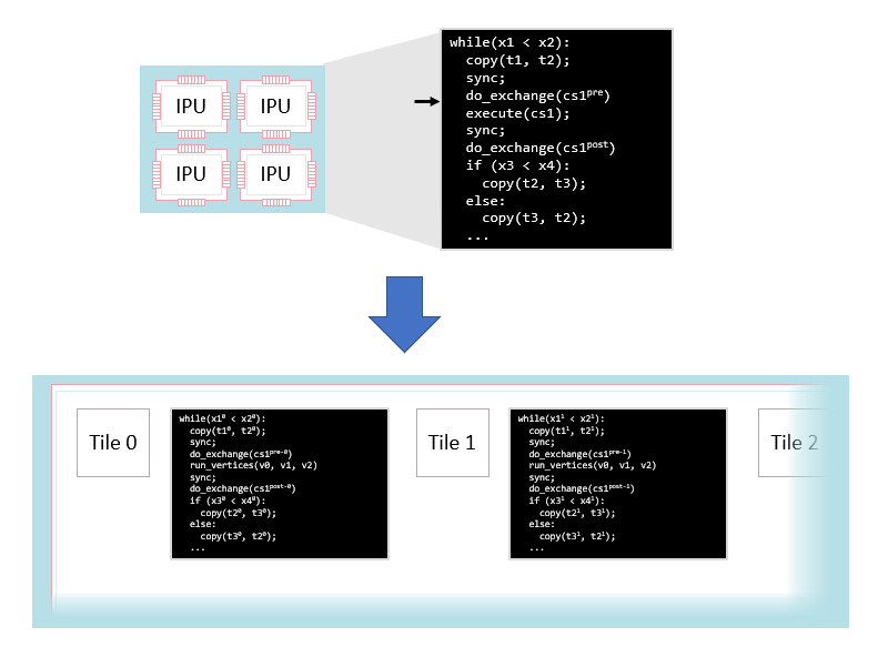
Fig. 3.14 Lowering a program to multiple tiles
After this lowering, each tile has its own version of the program. This version:
Only reads and writes data in its own tile memory
Contains explicit synchronisation instructions to other tiles
Contains data communication routines to exchange with other tiles
Just runs that tile’s vertices when executing a compute set
This lowering is done by the Poplar graph library. The result is a per-tile program that can be compiled with a conventional compiler to run on the tile.
Note that although this lowering occurs, due to the synchronisation between tiles it is still possible to view the execution as a global execution across all the tiles. This is the view the PopVision Graph Analyser tool shows, for example.
3.5.1. Variable liveness
Within the program, all the variables are global. The variables are stored either in Streaming Memory or across the tile array (where they will have multiple addresses in tile memory for each region of the variable stored on different tiles).
Despite the global scope of the variables, the variables do not all have distinct addresses for their regions in tile or Streaming Memory — they can overlap and some variables will share the same region of memory. This is possible because the inputs and outputs of each step of the program are known and so the liveness of each variable (that is, at which points in the execution of the program the variable is needed) is known during compilation. This allows the compiler to allocate variables that are not live at the same time to the same memory address.
At each point during program execution, a number of the variables will be live. This is equivalent to the size of a memory heap in dynamically allocated systems. The live variable memory size is the amount of temporary memory being used at that time. Some variables are always live — they always contain data that may be used later and these will have distinct addresses in memory.
The PopVision Graph Analyser shows the live memory and alway live memory as a program executes. The following snapshot shows this to give an idea of how memory usage varies during program execution.
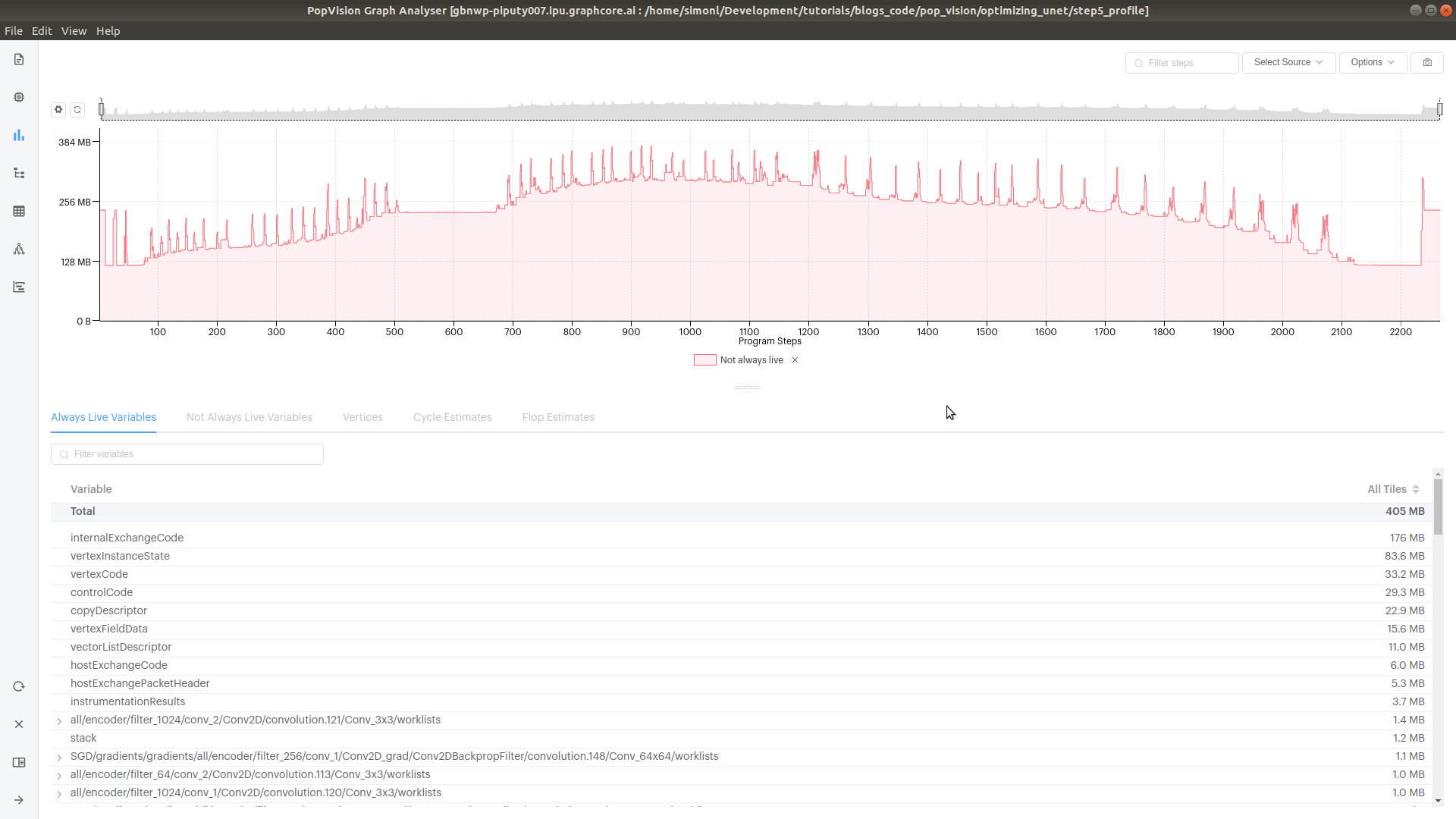
Fig. 3.15 Live variable memory over time