4. Optimising for performance
This section describes the various factors that affect ML model performance and under what conditions they are applicable.
4.1. Memory
Generally, more efficient memory use will translate into performance improvements during training and inference. Better optimised memory means larger batch sizes can be used, thus improving the throughput in both inference and training. Large operations that need to be serialised over multiple steps, for example, matmul and convolutions, can be executed in fewer cycles when more temporary memory is available. When more In-Processor-Memory is available, this reduces the need to access the slower streaming memory.
Section 5, Common memory optimisations describes the methods used in memory optimisation in detail.
4.2. Pipeline execution scheme
Good for |
Training large models |
|---|---|
Training with large global batch sizes |
|
Not recommended |
Low-latency inference |
The most common execution scheme for large models on the IPU is pipelining. This is a form of model parallelism, where a large model is split into multiple stages running on multiple IPUs. Each IPU contains a portion of the model and the IPU utilisation is maximised by running a pipeline of data. Once a pipeline is established there is always more than one micro-batch “in flight”.
The pipeline efficiency is bound by the longest stage executed at any one time. There is thus no point in optimising a pipeline stage if its length is dominated by a longer one. Performance gains can also be achieved by “breaking up” the longest stage and re-balancing it over all pipeline stages.
Pipelining works best when the gradient accumulation factor is much greater than the number of stages, since \(2 N\) stages are always under-utilised during the ramp up and ramp down phases of the pipeline.
During training, pipelining provides two options for the arrangement of the forward and backward passes:
grouped
interleaved.
Note these pipeline schedule options may not be available in all frameworks.
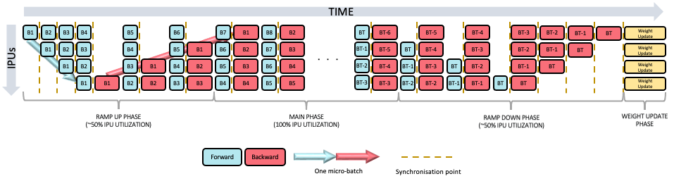
Fig. 4.1 Grouped pipeline schedule.
Grouped scheduling (used by default, Fig. 4.1) is generally faster but requires more memory to stash the activations than the interleaved scheduling.
Grouped scheduling requires storing:
\(2 N+1\) activations stored in FIFOs on the first IPU
\(2 (N-1)+1\) activations stored in FIFOs on the second IPU
and so on.
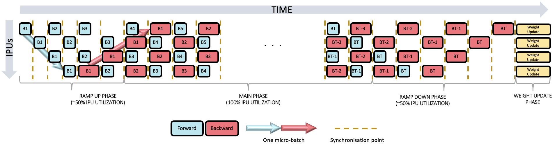
Fig. 4.2 Interleaved pipeline schedule.
Conversely the interleaved scheduling (Fig. 4.2) uses less memory to store the activations but may be slower, since a backward pass, generally longer than the forward pass, is always executed at every stage of a pipeline.
Interleaved scheduling requires storing \(N+1\) FIFOs of activations.
Pipelining generally comes with recomputation of activations, which is described in Section 5.3, Activation recomputations.
Available resources for pipelined execution:
4.3. Data parallelism
In cases where the model is small enough, but the dataset is large, the concept of data parallelism may be applied. This means that the same model is loaded onto each IPU, but the data is split up between IPUs. Data parallelism is the most common way to perform distributed training.
Good for |
Small-ish models (fit on few IPUs) |
|---|---|
Not recommended |
Heavy host I/O and preprocessing |
4.3.1. Graph replication
Data parallelism is achieved by replication of the Poplar graph.
Each replica operates on a micro batch. During inference, the results from each replica are enqueued in the Poplar outfeed queue and sent to the host.
During training via backpropagation, the gradients {\(g_{i}^{n}\}\) are calculated independently on each replica \(n\) and then reduced across all replicas before performing the weight update.
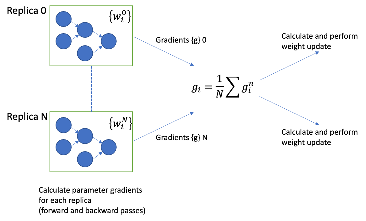
Fig. 4.3 Calculation of gradients across replicas and weight updates during training.
Note the weights are not explicitly shared yet they remain consistent (\(w_{i}^{0} = w_{i}^{1} = \ldots = w_{i}^{N}\)) across all replicas by sharing the same weight updates. Therefore, the weights must be initialised to the same value on each replica.
Replicas typically span multiple IPUs or even IPU-Machines or Pod systems. The cross-replica reduction introduces more communication across multiple IPUs and introduces a performance overhead. The relative impact of the communications overhead can be reduced by using a larger replica batch size, typically by increasing the gradient accumulation.
Using replication also increases the exchange code, linearly with the number of replicas, as illustrated in Table 4.1. Note that increasing the number of replicas from 1 to 4 (in Table 4.1) has increased the size of the global exchange code by a factor of 4. In this application the size of the global exchange code is still negligible when compared with the size of the internal and host exchange code.
1 Replica |
4 Replicas |
|
|---|---|---|
Control Code |
91,668,904 Bytes |
117,063,756 Bytes |
Internal exchange Code |
108,270,156 Bytes |
126,520,640 Bytes |
Host exchange Code |
66,044,276 Bytes |
66,147,360 Bytes |
Global exchange Code |
1,035,988 Bytes |
4,657,516 Bytes |
You can enable local replication in different frameworks:
However, for better scaling performances it is recommended to use PopDist and PopRun when possible.
4.3.2. Multiple SDK instances and replication: PopDist
One challenge that may arise when using graph replication is that the throughput performance stops increasing with the addition of new replicas because of the host limited compute power and bandwidth. For example the model can become CPU-bound from JPEG decoding or data augmentation on the host.
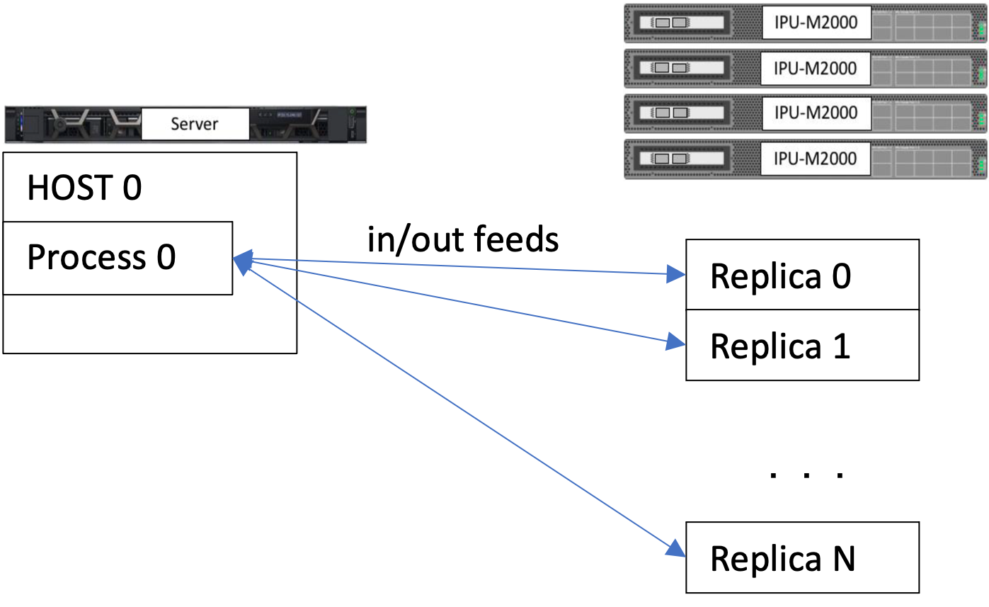
Fig. 4.4 A single instance of the host Poplar SDK feeding into multiple replicas of the graph.
This situation can be improved by using PopDist, which distributes the host-side processes on multiple processors or even hosts. PopDist relies on MPI to seamlessly allow graph replication to use multiple hosts and instances. Two common improvements are:
Increasing the number of host processes (which share the same I/O connectivity), if the application is compute bound by the host preprocessing
Increasing the number of hosts (vertical scaling), if the application is also I/O bound.
In Fig. 4.5, each process is an
instance of the host code run by PopRun and is connected to a single instance
of the replicated model. The preprocessing and I/O communications happen inside
the host processes.
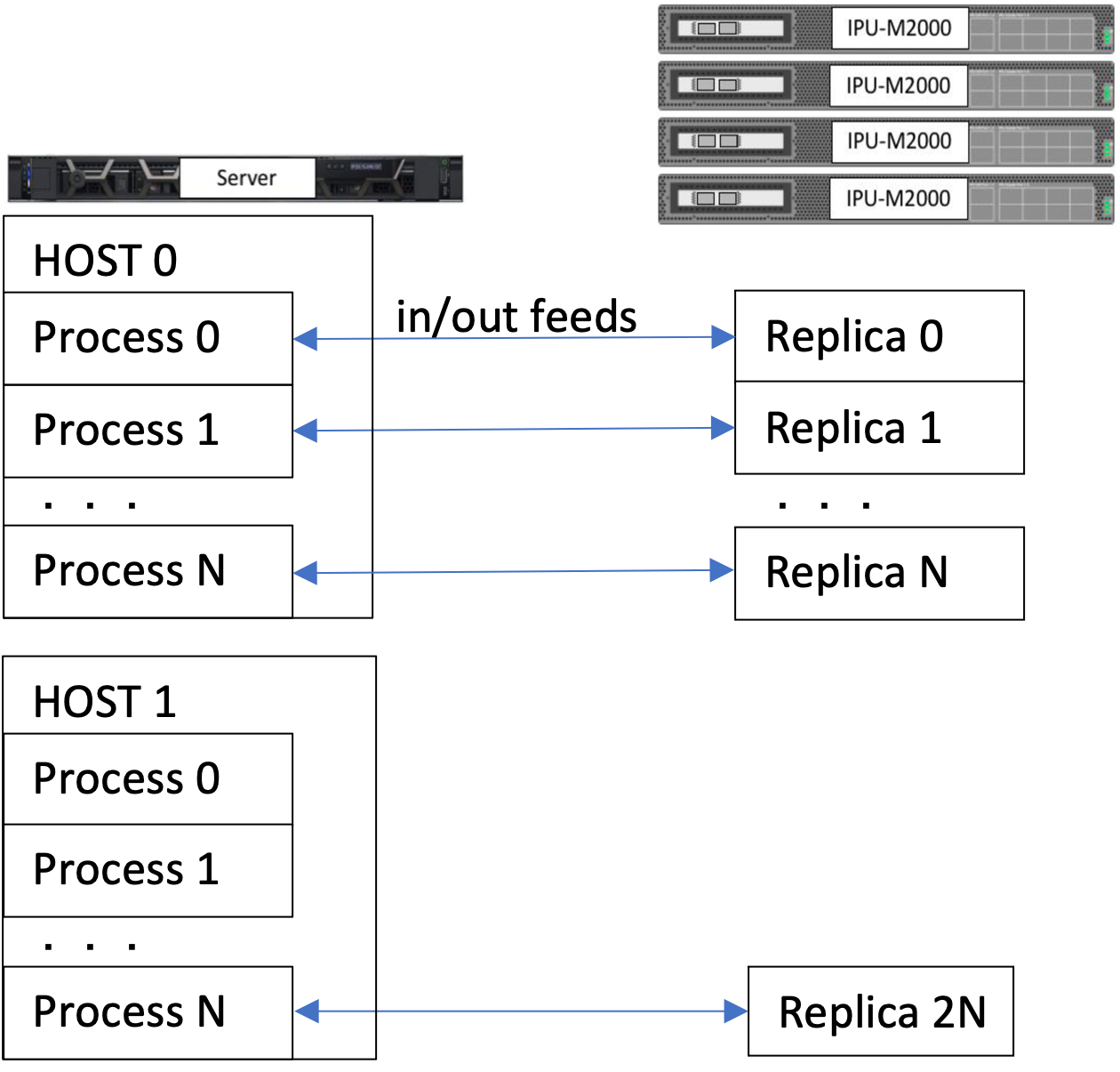
Fig. 4.5 With PopDist, multiple instances of the programs, possibly distributed over multiple hosts, can feed into multiple replicas of the graphs.
Code examples for PopDist:
4.4. Host-IPU I/O optimisation
Good for |
I/O-bound models |
|---|---|
Not recommended |
Model memory requirements are close to the IPU maximum memory |
How memory external to the IPU is accessed affects performance. Data is transferred in streams, with the IPU using a callback function to indicate to the host that the host can read data from the buffer (for IPU to host transfer) and that the host can populate the stream (for host to IPU transfer). For more information about data streams, refer to the Poplar and PopLibs User Guide.
There are three options that can be used to maximise I/O performance:
Prefetch depth
I/O tiles
Reducing the bandwidth required, for example, by using 8-bit integers or FP16 transfers.
4.4.1. Prefetch and prefetch depth
Enabling prefetch means that the IPU should call the callback function as early as possible (for example, immediately after it releases the stream buffer from a previous transfer). The host is then able to fill the buffer in advance of the transfer, meaning the IPU spends less time waiting for the host because the data is available before it is needed. The prefetch depth controls how much data is fetched, and a prefetch depth of 3 seems optimal.
To modify the prefetch depth:
Tensorflow provides a prefetch_depth option for the
IPUInfeedQueue.PopART also provides a way to change this value with the session option
defaultPrefetchBufferingDepth.PopTorch has direct access to certain advanced PopART options:
opt = poptorch.Options()
opt._Popart.set("defaultPrefetchBufferingDepth", 3)
4.4.2. Overlapping I/O with compute
The option to designate a number of IPU tiles to be I/O tiles allows for the Poplar graph to be constructed so that the data transfer and the computation can overlap in time.
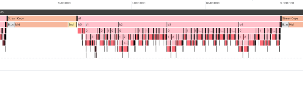
Fig. 4.6 No I/O tiles designated. The StreamCopy happens before execution of the model code.
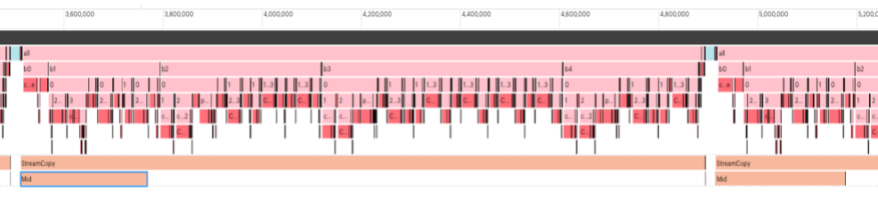
Fig. 4.7 Using I/O tiles. StreamCopy happens in parallel with the execution of the model code.
Setting the number of IO tiles is left up to you and depends on the application. The IO tiles must hold at least a full micro-batch of data and not all the memory on an IO tile is available for data (typically ~5% is used for the exchange code and buffers). Thus a rule of thumb for the number of IO tiles (\(N_{IO}\)) to allocate is:
\(N_{IO} \approx 1.05*\frac{S_{micro\_ batch} \cdot S_{micro\_ batch}}{S_{tile}}\)
where \(S_{micro\_ batch}\) is the micro-batch size and \(S_{tile}\) = 624 kB on the Mk2 IPU.
It may be more optimal if the number of I/O tiles is a power of 2, and doing a sweep of values that are a power of 2 is recommended. Note that, as of SDK 2.3, this will only overlap I/O with computation for a single IPU application or a pipelined application using the grouped schedule. Also, for a multi-replica or multi-instance configuration, the host multi-threading must be configured with the Poplar engine runtime options:
streamCallbacks.multiThreadMode: collaborative
streamCallbacks.numWorkerThreads: 6
Documentation for I/O tile settings:
4.4.3. Data size reduction
Instead of transferring the data in single-precision floating point (FP32) format, it is possible to improve data throughput by transferring the data in half-precision floating point (FP16) or, if possible, in Int8 format. The latter is especially relevant for images, where data normalisation/scaling happens on the accelerator instead of the host. Similarly, the returned data can be reduced if it requires a large portion of the bandwidth.
4.4.4. Disabling variable offloading
As explained in Section 5.4, Variable offloading, the optimiser state parameters can be offloaded to the host during training to save IPU memory. Sometimes, this variable offloading can cause a significant decrease in throughput performance. Here are the steps you should follow to identify and potentially prevent this from happening in your model:
With executable caching disabled and graph profiling enabled, perform a short training run with your model and open the generated profile in PopVision Graph Analyser.
In the Execution Trace, zoom in so that one iteration of your model is visible. Looking at the summary at the bottom of the window, evaluate whether the percentage of cycles used for “StreamCopyMidRemoteBuffer” is significant.
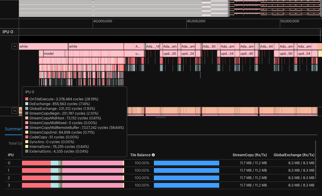
Fig. 4.8 Execution Trace and summary with default variable offloading. In this example “StreamCopyMidRemoteBuffer” is consuming >58% of the cycles.
If the percentage of cycles used is significant, try disabling variable offloading and retest your model. If you were near the memory limit, then this may trigger an
Out of Memoryerror. If not, then you should see a dramatic decrease in the cycles consumed copying to and from these optimiser state remote buffers and therefore an increase in throughput.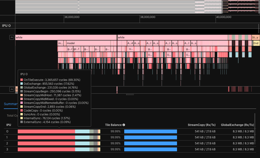
Fig. 4.9 Execution Trace and summary with variable offloading disabled.
4.5. Host-side processing optimisations
4.5.1. Host and IPU preprocessing
You can improve your data pipeline with caching and more efficient preprocessing, for example, normalisation of the data, or you can move some of the preprocessing directly to the IPU. This makes sure that data is generated fast enough.
4.5.2. The one-computational-graph concept
The Graphcore frameworks extract the computational graphs from different frameworks like PyTorch and TensorFlow and post-process them to obtain highly efficient computational graphs that get executed on the IPU. Since the IPU looks at the whole graph and not just single operators, this compilation process can take a bit longer. Thus, we provide features like executable caching in the different frameworks to make sure that compilation happens rarely and loading the executable to hardware takes very few seconds.
However, when developing the application code, it is important to avoid changing the computational graph because this will trigger recompilation when the change occurs for the first time and later on it will trigger changes of the executable. Hence, it is preferable that there is only one computational graph. A common example that creates more than one graph is when the batch size changes. With a different batch-size, data and compute need to be distributed differently to the IPU tiles and thus a new optimisation is required. Further examples are provided in the technical note Optimising for the IPU: Computational Graph Recompilation and Executable Switching in TensorFlow. Similarly, eager execution breaks down the full graph into multiple subgraphs, which should be avoided as described in the TensorFlow 2 user guide.
4.5.3. Looping
Instead of processing sample by sample, it is beneficial to loop over streams of samples instead. In this way, data is continuously transferred between host and device and the host-side overhead of starting and stopping the processing process is avoided. This happens in most of our interfaces. For example to loop in TensorFlow Keras, use steps_per_execution or to loop in PyTorch use deviceIterations.
However, in some TensorFlow applications, processing still needs to happen sample by sample. In these cases, explicit loops should be used, as shown in the TensorFlow 2 porting examples.
4.6. Optimising numerical precision
Good for |
Most deep learning models |
|---|---|
Not recommended |
May need some granularity to avoid loss of precision in critical parts of the model |
Reducing the numerical precision is a common way to improve the training or inference performance of a model. This uses less memory for all operations, increases the bandwidth of data exchanges, and reduces the number of cycles required by arithmetic operations.
Note that numerical stability issues may arise when reducing the numerical precision. While resolving these issues is out of the scope of this document; some key ideas are:
Using loss scaling when the gradients are calculated in reduced precision. This will limit the risk of underflow errors when gradient values are too small to be accurately represented.
Enabling stochastic rounding to improve the average numerical accuracy, in particular during weight update.
How to enable it: Tensorflow | PyTorch | PopART
Analysing the distributions of the values of the weights and gradients in all layers of the networks, and locally increasing the precision of some critical operations.
For more information on numerical precision on the IPU, refer to the AI Float White Paper.
Additional resources for half-precision training:
4.7. Replicated tensor sharding (RTS)
Good for |
Very large models |
|---|---|
Large number of optimiser states |
|
Not recommended |
Models without data parallelism |
Exchange bandwidth already constrained by data I/O |
Replicated tensor sharding is a technique only available in combination with graph replication. With replicated tensor sharding, a tensor that would otherwise contain the same information on all replicas can be sharded (for example, broken up into equal sub-tensors) across all replicas of a graph. This frees up memory on the replica, but requires re-assembling the tensor when it needs to be used.
This feature can be utilised with tensors both on (stored in IPU SRAM) and off chip (stored in Streaming Memory).
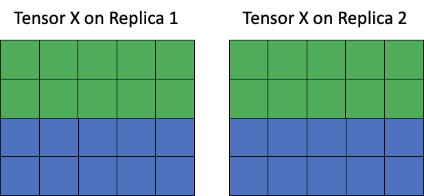
Fig. 4.10 Tensor memory layout before sharding
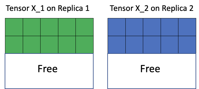
Fig. 4.11 Tensor memory layout after sharding
Replicated tensor sharding is especially useful for sharding the optimiser states across replicas. This enables you to apply the optimiser update in parallel across many replicas. Each optimiser update then only acts on its corresponding shard of the parameters before reducing over the replicas. This requires additional operations and so is more beneficial on large, distributed models, where the trade-off between these operations is outweighed by the benefits of parallelism.
This method is similar to Microsoft’s Zero Redundancy Optimizer (ZeRO).
Enabling replicated tensor sharding:
In Tensorflow, CrossReplicaGradientAccumulationOptimizerV2 and GradientAccumulationOptimizerV2 take an optional argument
replicated_optimizer_state_sharding. This will shard the optimiser state tensors among replicas. It can also be set when using the pipelining Op . When using multiple instances, the tensor is partitioned across the local replicas owned by each process. Each host instance has access to the complete variable tensor.PopART provides a flexible tensor location API to configure RTS.
Since PopART is the backend for PopTorch, the PopART logic applies for RTS in PopTorch. The tensor location options can be accessed via poptorch.Options.TensorLocations.
For instance, let’s set RTS for the optimizer state tensors as soon as it contains more elements than our number of replicas. Let’s assume we are using PopDist and PopRun to handle distributed training.
In PopART:
opts = popart.SessionOptions()
popdist.popart.configureSessionOptions(opts)

num_local_replicas = popdist.getNumLocalReplicas()
opts.optimizerStateTensorLocationSettings.minElementsForReplicatedTensorSharding = num_local_replicas
opts.optimizerStateTensorLocationSettings.location.replicatedTensorSharding = popart.ReplicatedTensorSharding.On
In PopTorch:
opts = popdist.poptorch.Options()

num_local_replicas = popdist.getNumLocalReplicas()
opts.TensorLocations.setOptimizerLocation(
   poptorch.TensorLocationSettings()
   .minElementsForReplicatedTensorSharding(num_local_replicas)
   .useReplicatedTensorSharding(True)
)
Note
PopART’s
CommGroupsettings are not available in PopTorch. PopTorch usesCommGroupType.Consecutiveas default: Tensors are sharded among the local replicas. Each host instance has access to the complete variable tensor.
4.8. Tile mapping
A poor tile mapping can lead to strided copying. Strided copying arises when either the memory access patten or the location in memory of data is non-contiguous, for example, when you are transposing data. This leads to slower performance and has a considerable code cost.
There are two ways you can identify that strided copying exists:
Use the PopVision Graph Analyser tool to examine the list of vertex types. Strided copies will have names of the form
DstStridedCopyand there will be many of them.PopVision allows you to look at the program tree to track down where the vertices are used.
The execution graph shows many
PreArrangesteps, likePreAarrange-0andPreArrange-1.These indicate on-tile copy operations which rearrange data. The data is rearranged so that it has the correct layout for input to vertices, for example, for alignment and to make the input contiguous in memory.
Strided copies could also be the result of suboptimal mapping by the framework. One way to address them directly in the framework is to reverse the operands or to use PopLibs functions directly as part of custom operators. Refer to the technical note Creating Custom Operations for the IPU for details.
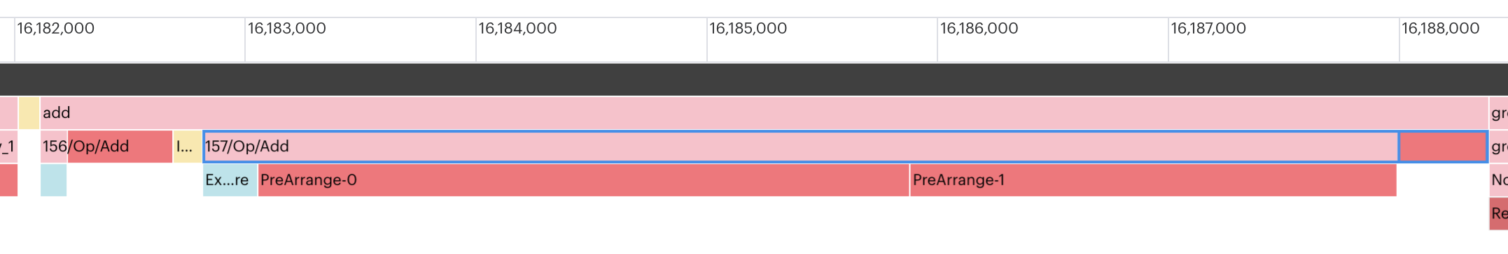
Fig. 4.12 PopVision execution trace showing PreArrange steps taking up significantly more cycles than the operation itself.
In this example the additional operation takes about 580 cycles while 5800 cycles are needed to re-arrange the tensors. (Note that Group Executions must be disabled in the Options of the Execution Trace plot.)
4.9. Other execution schemes
Good for |
Very large models |
|---|---|
Very large code |
|
Models with interdependencies between pipeline stages |
|
Not recommended |
This is generally not supported in high-level ML frameworks |
Other execution schemes, such as domain sharding and TensorParallel execution, can be considered as a “last resort” as they are not easily implemented at the application level.