10. Writing vertices in assembly

This chapter introduces the general concepts required for writing vertices in assembly code. For other Graphcore-specific terminology, see the Glossary.

Table 10.1 Terminology used in this document

Notation	Meaning
ARF	Auxiliary register file; the registers associated with the auxiliary execution pipeline.
Aux	The auxiliary execution pipeline.
Bundle	A group of instructions executed in parallel.
Context	The complete and distinct environment for a single thread of execution. Each tile supports a single supervisor context alongside a number of worker contexts. State, such as the registers, is replicated for each context.
CSR	Control and/or status register
LIW	Long instruction word. An architecture that executes multiple instructions in parallel.
Main	The main execution pipeline.
MRF	Main register file; the registers associated with the main execution pipeline.
Naturally aligned	Natural alignment is where the alignment of a data object in memory is equal to the data size.
PC	Program counter
SP	Stack pointer
Supervisor	A single execution context. The supervisor execution thread is responsible for: Initiating worker threads Performing the exchange and barrier synchronisation phases of a superstep. A single tile supports just one supervisor context. Supervisor code cannot perform some operations, most notably floating point. See the Tile Vertex Instruction Set Architecture for more information.
Worker	A single execution context. A worker execution thread is responsible for performing the computation phase of a superstep. A tile has hardware support for multiple worker contexts.

Table 10.2 Notation used in this document

Notation	Meaning
0xvalue	A value written using hexadecimal notation
0bvalue	A value written using binary notation
value	A value written using decimal notation
value[i]	Bit i of value
value[j:i]	Bits i through j of value
$SOME_STATE	Refers to tile architectural state, such as a register
$an	Register n in the arithmetic register file (ARF)
$mn	Register n in the main register file (MRF)

10.1. Instruction set overview

The instruction set architecture (ISA) of the tile processor, including the execution pipeline and registers, is described in detail in the Tile Vertex Instruction Set Architecture.

This section introduces some of the concepts that will be referred to in later chapters. For a high-level introduction to the IPU, please refer to the IPU Programmer’s Guide

The tile is a highly-deterministic, asymmetric, dual pipeline, long instruction word (LIW) processor. It supports multiple hardware resident execution contexts. These contexts are time multiplexed onto shared hardware resources to achieve high utilisation by hiding local instruction latencies, including memory access and branch latencies.

Each tile includes tightly-coupled local memory which is used to store all code and data required by the tile.

10.1.1. Supervisors and workers

An IPU tile has two types of hardware execution contexts: a supervisor context and six worker contexts. There are six execution slots that can run these contexts. A round-robin schedule is used to time multiplex the execution slots (and therefore active contexts) onto the shared hardware resources.

Initially, there is only a single supervisor thread that runs in all execution slots. When worker threads run they occupy a single execution slot. When six workers are running, the supervisor is suspended until an execution slot is made available by the termination of a worker.

The supervisor can only perform certain operations. For example, it cannot execute floating-point instructions.

Supervisor code is used for overall control of execution, synchronisation and exchanges, but all floating-point processing must be done in a worker context.

Workers can execute instructions individually or in parallel with another instruction as part of an execution bundle. A bundle consists of one instruction for the main pipeline and one for the aux pipeline (see Section 10.1.2, Execution pipelines).

You can access the Vertex state from assembly code. In the same way that you would expect the this variable in C++ to point to the first field inside a class, in a vertex function the equivalent pointer is available in the $mvertex_base register.

Vertices with base class Vertex have no parameters (all state is accessible through the register $mvertex_base). On termination they must provide an exit status using one of the exit instructions. They are not required to preserve any register state.

Vertices with base class MultiVertex have a single parameter to the MultiVertex::compute(unsigned) method which is the thread ID of the worker running the method. This value is available in the $WSR register. It must be masked out of the register which contains several bitfields packed together.

Vertex and MultiVertex vertices terminate via exitz or exitnz; when declared to return void they must exitz $mzero. Supervisor vertices terminate via a standard br $lr and return using the standard function return convention, so a bool can be returned in $m0.

get $m0, $WSR
and $m0, $m0, CSR_W_WSR__CTXTID_M1__MASK

The total number of invocations of the multi-vertex compute method is provided by the constant CTXT_WORKERS defined in poplar/TileConstants.hpp.

10.1.2. Execution pipelines

The tile has a pair of asymmetric execution pipelines, main and aux:

• Main is designed primarily to perform control flow, address manipulation, integer arithmetic and load/store operations

• Aux is designed primarily to perform floating-point based compute

A supervisor thread cannot use the aux pipeline and its associated state.

Each pipeline has an associated register file. The main execution pipeline is associated (and tightly coupled) with the main register file (MRF) and the aux pipeline with the auxiliary register file (ARF).

These register files, as well as control and status registers and some internal state, are replicated for each context.

The are 16 32-bit registers in the main and arithmetic register files. These are referenced by the names $mn and $an. Some of these registers have predefined functions and some are read only, as shown in Table 10.3. See the Tile Vertex Instruction Set Architecture for full details.

Table 10.3 Special registers

Register	Alias	Function	Read only
$m9	$fp	Frame pointer	N
$m10	$lr	Link register (return address)	N
$m11	$sp	Stack pointer	N
$m12	$mworker_base	Worker stack base	Y
$m13	$mvertex_base	Vertex stack base	Y
$m15	$mzero	Returns zero	Y
$a15	$azero	Returns zero	Y
$a14:15	$azeros	Returns 64-bit zero	Y

Note

The registers used as $fp, $lr and $sp are normal general-purpose registers and could be used for any purpose. Their special function is just a convention defined by the ABI. The other registers in the table have hardware-defined functions.

For full details of all the registers, see the Tile Vertex Instruction Set Architecture.

10.2. Memory architecture

The architectural size of the tile memory is limited to 21 address bits (2 MB). The tile memory is the only memory directly accessible by tile instructions. It contains both the code and data used by that tile. There is no shared memory access between tiles.

The tile uses a contiguous unsigned 21-bit address space, beginning at address 0x00000. Every context, both worker and supervisor, has visibility of the entire address space. In practice, only a part of this memory space is populated with memory. The physical memory has a non-zero start address as a simple way to prevent invalid zero-valued addresses from being accessed. Attempting to access an unpopulated memory address will cause an exception.

The memory is organised as two regions, each made up of a number of 64-bit wide banks. Concurrent accesses can be made to addresses in different banks. This allows, for example, a 64-bit instruction fetch and two 64-bit data accesses to occur simultaneously (one may be a write).

Accesses to the banks in region 1 are interleaved, with bit 3 of the address selecting 64-bit words from alternating odd and even banks. A pair of banks containing interleaved addresses form a single 128-bit wide memory element.

Interleaving allows for two 64-bit aligned addresses, a and a+8, to be accessed simultaneously. This enables, for example, a 128-bit load and a simultaneous 64-bit load or store. Such simultaneous accesses would cause a memory clash exception in the non-interleaved memory region (unless the two addresses happened to straddle the boundary between two banks).

Instructions can only be fetched from region 0. Attempting to execute code from interleaved memory will cause an exception.

For more information, see the “Memory model” chapter in the Tile Vertex Instruction Set Architecture.

10.2.1. Getting information about the memory

The Poplar API provides details of the hardware that the software is actually executing on.

• Target::getBytesPerTile() function returns the size of tile memory in bytes.

• getMemoryElementOffsets() returns an array containing the offsets, from the start of memory, of each of the elements (not banks). For the Mk2 Colossus, for example, this will return 26 values, corresponding to the thirteen 16 KB elements and thirteen 32 KB elements.

• getInterleavedMemoryElementIndex() returns the index of the first element in interleaved memory (for Mk2 Colossus, for example, this will return 13).

Details of these and other related functions can be found in the Poplar and PopLibs API Reference.

10.2.2. Mk2 Colossus (GC200)

In the Mk2 Colossus, each tile has 624 kilobytes of SRAM (see Fig. 10.1). This means that an IPU with 1,472 tiles has just under 900 MB of memory in total.

The available memory starts at address 0x4C000 and ends at 0xE7FFF.

Table 10.4 Memory organization for Mk2

Region	Size	Interleaved	Banks (16 KB)	Elements (size)
0	208 KB	N	13	13 (16 KB)
1	416 KB	Y	26	13 (32 KB)

Region 0 is selected when bit 19 of the address is 0, and is addressed with bits [18:3]. Bits [18:14] select the bank, or memory element, and bits [13:3] select a 64-bit word from that bank.

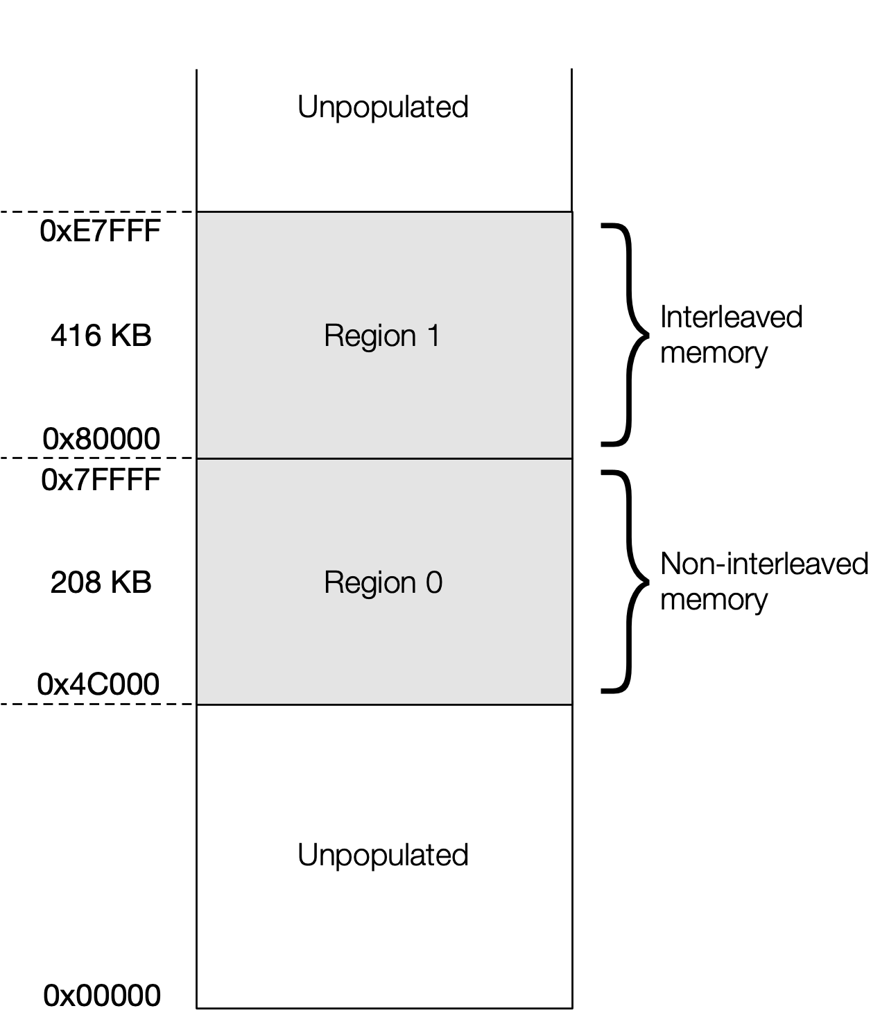
Fig. 10.1 Memory architecture for Mk2 Colossus

10.2.3. Load and store instructions

There are load instructions for the following data sizes:

• 8 bit

• 16 bit

• 32 bit

• 64 bit

• 128 bit (only from region 1)

And store instructions for the following data sizes:

• 32 bit

• 64 bit

There are instructions that can perform multiple simultaneous loads, as well as instructions that do a simultaneous load and store.

If you try to make more than one access to a memory bank in one cycle you will get a memory conflict. Interleaved memory places sequential 64-bit words in alternating banks, allowing you to use more efficient load-store instructions like ld128, ld2xst64pace, etc. See Section 10.4, Vertex pipelines for an example of their use.

All loads (including instruction fetches) and stores must be naturally aligned. Misaligned accesses will result in an exception.

10.3. Worker stack and scratch space

The codelet is allocated a stack and a small “scratch space”, which can be used for temporary storage.

The stack and scratch space are arranged as shown below.

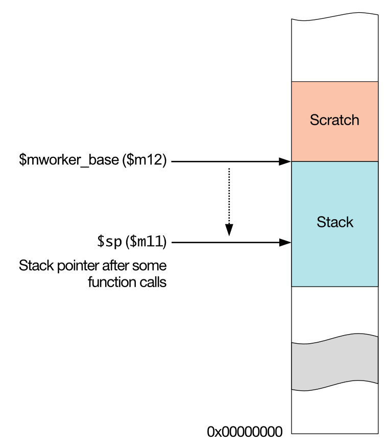
Fig. 10.2 Stack memory layout

The register $mworker_base (an alias for $m12) is a read-only register that is initialised to the top of the stack, which is also the bottom of the scratch space. The stack pointer, $sp (an alias for $m11), is not initialised. If you want to use the stack you must initialise $sp to ($mworker_base - stack_allocation_size) before storing objects on the stack.

Any functions that are called will need to allocate stack by adjusting the stack pointer, for example to allocate 32 bytes of stack for a function:

add $sp, $sp, -32

The stack space will need to be deallocated before the function returns.

If your code does not need any stack space, you can directly store items in the scratch space using $mworker_base and use $m11/$sp as a general purpose register instead.

The size of the scratch space is defined by poplar::WORKER_SCRATCH_SIZE in Engine.hpp. This cannot be changed.

The size of the stack needs to be defined for each function as described below.

10.3.1. Specifying stack size

When C++ functions are compiled, the compiler is usually able to determine the stack required. This is not possible for assembly code so you must explicitly specify the stack used by your functions. This enables the Poplar runtime software to determine the total stack usage when it builds the graph.

Note that C++ versions of these macros are also provided for those cases where the compiler is not able to determine the stack space required

Note

If the stack usage for an assembly function is not specified (or is specified more than once) then graph compilation will fail with an exception.

If the stack usage is wrongly specified (that is, smaller than required) then this can result in a stack overflow at run time. This will not be detected (stack overflow detection works only for C++ codelets) and may cause errors that are hard to debug.

A couple of macros are provided for specifying the stack size of functions. These are defined in the Poplar header file StackSizeDefs.hpp which you will need to include in your source file. See the runtime API section of the Poplar API Reference for more information.

• DEF_STACK_SIZE_OWN size function

  This defines the stack size (in bytes) used only by the specified function. The Poplar runtime will traverse the call graph (the tree of all functions called, with the root being the specified function) to calculate the total stack required. You will also need to explicitly define the stack size of all functions called (or jumped to) by function.

  Note that if the assembly function calls library or other C++ functions then you must use this macro and not DEF_STACK_USAGE.

• DEF_STACK_USAGE size function

  This defines the total stack usage (in bytes) for the function specified and any functions that it calls. In this case, Poplar will not traverse the call graph of the function and you do not need to specify the stack usage of the functions called by function.

Most assembly vertices don’t use a stack and have a simple code structure so the DEF_STACK_USAGE macro is often all you need.

The top-level entry point in the assembly vertex (the __runCodelet_XXXXX function) always needs to be marked with one of the two macros, even if the stack size is zero.

In these macros, you can specify function as either a function name or a section name.

If each function is contained in its own section (as it should be, so that the Poplar runtime can remove unused code) then it makes no difference whether you specify the function name or the section name.

If you specify a section name and that section contains multiple functions then size is the maximum stack space used by any of the functions in the section.

10.3.2. Examples

1. A codelet that uses no stack space at all:

DEF_STACK_USAGE  0  __runCodelet_XXXX

This specifies that the Poplar runtime does not need to look at the call graph of the function, as no stack used. This may be the most common case.

2. A codelet using N bytes of stack space in total:

DEF_STACK_USAGE  N  __runCodelet_XXXX

Again, the Poplar runtime does not need to look at the call graph of the function, as the stack usage is fully specified.

3. A codelet function that uses N bytes of stack space itself, but which calls other functions. The assembler will need to traverse the call graph to compute the total stack usage:

DEF_STACK_SIZE_OWN  N  __runCodelet_XXXX

10.4. Vertex pipelines

A tile can simultaneously execute memory and arithmetic operations in a single cycle using an instruction bundle. You can double the performance of some loops if you can arrange the instructions to take advantage of this.

For example, consider a function that adds a value to all the elements of an array. The code for this, using vectors of two-floats, is:

float2 addend = ...;
float2* acts = ...;
for (unsigned i = 0; i < N; ++i)
    acts[i] += addend;

In other words:

1. Load 64 bits of acts (two floats).

2. Add the two addend floats to them.

3. Store them back and increment the acts pointer by 64 bits.

4. Loop.

A simple implementation using a rpt loop is shown below. The rpt instruction takes two operands: a loop count (which can be an immediate or a register) and the length of the loop body, which follows the instruction.

  rpt $N, (2f - 1f)/8 - 1
1:
  {
    ld64 $tmp0, $mzero, $acts, 0
    fnop
  }
  {
    nop
    f32v2add $tmp0, $tmp0, $addend
  }
  {
    st64step $tmp0, $mzero, $acts+=, 1
    fnop
  }
2:

This works, but look at all those nop instructions. We can do better. First, there are instructions that do both a load and a store in one cycle. This means we can load the next 64 bits of addend at the same time as storing the previous 64 bits by using the ldst64pace instruction. That also provides control over how the pointers are incremented.

Second, we can put the f32v2add in the same bundle as the ldst64pace. So we want our unrolled loop to be something like this:

...
{
  ldst64pace .... // tmp = acts[i]
  f32v2add   ....
}
{
  ldst64pace ....
  f32v2add   .... // tmp += addend
}
{
  ldst64pace .... // acts[i] = tmp
  f32v2add   ....
}
...

Here, the load-store instruction in each bundle stores the result of the add from the previous bundle, and loads the data for the add in the following bundle. In other words, the load instruction is fetching data two words ahead of the store instruction.

We can implement this as a loop:

  rpt ..., (2f - 1f)/8 - 1
1:
  {
    ldst64pace $tmp0, $tmp0, $acts_packed+=, $mzero, 0
    f32v2add $tmp1, $tmp1, $addend
  }
  {
    ldst64pace $tmp1, $tmp1, $acts_packed+=, $mzero, 0
    f32v2add $tmp0, $tmp0, $addend
  }
2:

The register $acts_packed contains both the load and store addresses.

Unrolled, ths loop would effectively execute this:

{
  acts[0] = tmp0, tmp0 = acts[2]
  tmp1 += addend   // acts[1]
}
{
  acts[1] = tmp1, tmp1 = acts[3]
  tmp0 += addend   // acts[2]
}
{
  acts[2] = tmp0, tmp0 = acts[4]
  tmp1 += addend   // acts[3]
}
{
  acts[3] = tmp1, tmp1 = acts[5]
  tmp0 += addend   // acts[4]
}
...

If you look at acts[2], it is loaded in the first bundle, added in the second, and then stored in the third. We aren’t handling the beginning or end of the loop correctly yet, we’ll come back to that. Just think about the loop body for now.

10.4.1. Memory conflicts

This code looks like it would work, and it almost does. But if you try to execute it you will get a memory conflict exception. This is because concurrent loads or stores must be done to different memory banks.

Using interleaved memory (see Section 10.2, Memory architecture) can help in many cases, because alternate 64-bit words are in different memory banks. That means a 128-bit load can be done in one cycle, or a load-store instruction can store to one word and simultaneously read from the following word.

However, in our loop the loads and stores are two words apart. We store to the 64-bit word i at the same time as loading from i+2, which is 16 bytes offset from it. This means that these are in the same memory bank, even in interleaved memory.

10.4.2. Modified pipeline

To make use of the interleaved memory banks, the store needs to be delayed by an extra cycle. This means we need need to add a stage to the pipeline.

So, instead of this pipeline:

Cycle	Load	Add	Store
0	0
1	1	0
2	2	1	0
3	3	2	1
4	4	3	2
5	5	4	3
6	6	5	4
7		6	5
8			6

We do this:

Cycle	Load	Add	Store
0	0
1	1	0
2	2	1
3	3	2	0
4	4	3	1
5	5	4	2
6	6	5	3
7		6	4
8			5
9			6

This requires additional temporary values. We can implement this as shown below in pseudo-code:

rpt {
  {
    acts[0] = tmp0, tmp0 = acts[3]
    tmp2 += addend
  }
  {
    acts[1] = tmp1, tmp1 = acts[4]
    tmp0 += addend
  }
  {
    acts[2] = tmp2, tmp2 = acts[5]
    tmp1 += addend
  }
}

Or in assembly:

  rpt ..., (2f - 1f)/8 - 1
1:
  {
    ldst64pace $tmp0, $tmp0, $acts_packed+=, $mzero, 0
    f32v2add $tmp2, $tmp2, $addend
  }
  {
    ldst64pace $tmp1, $tmp1, $acts_packed+=, $mzero, 0
    f32v2add $tmp0, $tmp0, $addend
  }
  {
    ldst64pace $tmp2, $tmp2, $acts_packed+=, $mzero, 0
    f32v2add $tmp1, $tmp1, $addend
  }
2:

And now it works. In some cases you may not need to use explicit temporary values. For example, instead of using f32v2add we could use f32v2axpy which uses an internal accumulator as a temporary value.

The instruction f32v2axpy $dst, $src0, $src1 performs the following two operations simultaneously (it effectively has an internal 1-stage pipeline):

• $dst = $internal_accumulator

• $internal_accumulator = $TAS * $src0 + $src1

$TAS is a scale register. You can set it to 1.0 if you just want addition.

We can use this to simplify our loop to the following:

  rpt ..., (2f - 1f)/8 - 1
1:
  {
    ldst64pace $tmp1, $tmp1, $acts_packed+=, $mzero, 0
    f32v2axpy $tmp0, $tmp0, $addend
  }
  {
    ldst64pace $tmp0, $tmp0, $acts_packed+=, $mzero, 0
    f32v2axpy $tmp1, $tmp1, $addend
  }
2:

This saves eight bytes, and more importantly frees up an ARF register.

10.4.3. Fill and drain

Until now we have ignored the start and end of the loop. In practice we must take special care with filling and draining the pipeline because:

1. We don’t want to write junk before the start of our output array.

2. We don’t want to process junk after the end of our input array.

Note that it is ok to read junk after the end of our input array. However processing it (for example, with f32v2axpy) may raise a floating point exception. Also, although we can read past the end of our data, we can’t read past the end of the tile’s memory space, so depending on your alignment, stride, etc. you may need to avoid any over-reading.

Therefore, we essentially need to duplicate the loop body a few times before and after the loop, but changing the ldst64pace as appropriate to avoid extra reads and writes. For example:

  // Copy the address of the start of the acts as the store address, and
  // the load address for the pipeline fill stage.
  mov $mscratch0, $acts

  // Cycle 0:      Load 0
  ld64step $tmp0, $mzero, $mscratch0+=, 1

  // Cycle 1:      Load 1    Add 0
  {
    ld64step $tmp1, $mzero, $mscratch0+=, 1
    f32v2axpy $azeros, $current_addend0, $tmp0
  }

  // Cycle 2:      Load 2    Add 1
  {
    ld64step $tmp0, $mzero, $mscratch0+=, 1
    f32v2axpy $tmp1, $current_addend0, $tmp1
  }

  // First address is the load pointer. Second is ignored. Third is the
  // store pointer.
  // By using ld64step above we have set $mscratch0 to $acts+24
  tapack $acts_packed, $mscratch0, $mzero, $acts

  // We do two of the C loop bodies, in each rpt body, so divide N by 2.
  shr $rpt_count, $N, 1

  rpt $rpt_count, (2f - 1f)/8 - 1
1:
  {
    ldst64pace $tmp1, $tmp1, $acts_packed+=, $mzero, 0
    f32v2axpy $tmp0, $tmp0, $addend
  }
  {
    ldst64pace $tmp0, $tmp0, $acts_packed+=, $mzero, 0
    f32v2axpy $tmp1, $tmp1, $addend
  }
2:

  // We may need 1 or 2 more stores depending on whether or not $N is odd.
  and $mscratch0, $N, 0x01
  brnz $mscratch0, 1f
  // If it's even, do this:
  {
    st64pace $tmp1, $acts_packed+=, $mzero, 0
    f32v2axpy $tmp0, $addend, $azeros
  }
  st64pace $tmp0, $acts_packed+=, $mzero, 0
  bri 2f
1:
  // If it's odd, do this:
  {
    ldst64pace $tmp1, $tmp1, $acts_packed+=, $mzero, 0
    f32v2axpy $tmp0, $addend, $tmp0
  }
  {
    st64pace $tmp0, $acts_packed+=, $mzero, 0
    f32v2axpy $tmp1, $addend, $azeros
  }
  st64pace $tmp1, $acts_packed+=, $mzero, 0
2:

This example is even more complex because the loop body actually processes four floats per loop. So, if our array is 10 floats (for example), we need to add in another half of the rpt body at the end. Handling the ends of arrays can get tedious!

10.5. Assembly hints & tips

This chapter introduces some tips that may be useful when writing assembly code for the IPU.

This covers ideas related to assembly language, the IPU architecture and some more general comments.

10.5.1. Using the assembler

For full details of the assembler syntax and features please see the GNU Assembler Manual.

Assembler macros

The assembler supports macros which can be useful for avoiding code repetition, especially when creating versions of a vertex that use different types. The basic syntax is:

// Define a simple example macro
.macro GET_PARAMS VOFF_IN_PTR VOFF_OUT_START_PTR VOFF_OUT_END_PTR

  brz      $m0, dummy_label@
  ld32     IN_PTR, $mzero, $mvertex_base,VOFF_IN_PTR
  ld32     OUT_START_PTR, $mzero, $mvertex_base,VOFF_OUT_START_PTR
  ld32     OUT_END_PTR, $mzero, $mvertex_base,VOFF_OUT_END_PTR

dummy_label@: .endm

// Use the simple example macro

GET_PARAMS 0 1 2

This substitutes the parameters and inserts the generated code. The @ syntax simply inserts a number which increments each time any macro is used so the assembler produces unique labels which can be referenced within the macro. There are other useful assembler macro features, see the GNU assembler manual for details.

Labels

In assembly code you can define a label like this:

my_label:

Any use of the label refers to its address. So, for example, you can branch to a label like this:

bri my_label

my_label will become a symbol in the final ELF file. You can also create “local” symbols that can be jumped to within the file, but are not stored in the ELF symbol table. This is done by prefixing the label with .L

.Linfinite_loop:
  bri .Linfinite_loop

Here .Linfinite_loop will not appear in the symbol table.

Another useful trick is the labels 0: to 9:. These are also local labels: they do not appear in the symbol table.

0:
  bri 0b

However, you can use them multiple times. In order to specify one of these labels you append b or f. 0b means “the nearest 0: searching backwards” and 0f means “the nearest 0: searching forwards”. This is quite useful for short conditional blocks:

  // Set $b to 5 if $a is not 0.
  brz $a, 1f
  setzi $b, 5
1:

It is also useful for calculating the size of rpt bodies:

  rpt $n, (2f - 1f)/8 - 1
1:
  {
    ...
  }
  {
    ...
  }
  {
    ...
  }
2:

Recording the code size of the vertex

We recommended that you include a .size`size directive at the end of a function definition. This allows tools like ``objdump` to report the space used by the function. The information may be used by Poplar to choose between a faster specialisation or a smaller, general-purpose vertex.

This can be done as shown below:

myfunc:

  ...

.size myfunc, .-myfunc

Place each vertex in a unique section

With compiled code, you can use the linker option --function-sections to place each function in its own section and then remove unused sections for dead code elimination.

For functions written in assembly, the section needs to be specified explicitly. Each function should be in a different section with a name of the form .section .text.VERTEX_NAME, where VERTEX_NAME is the symbol of the function.

The same thing applies to data objects, they should be placed inside sections with names similar to .section .data.SYMBOL_NAME.

NOTE: new sections have a default alignment of 1 so you need to add a .align directive at the start of every section (either 4 or 8 depending on whether you have a rpt in your function or not).

10.5.2. Architectural tips

Aligning repeat bodies

A rpt body consists of a sequence of instruction bundles, and these must be 8-byte aligned. This is the only case where instructions must be 8-byte aligned (instruction bundles in general only need to be 4-byte aligned).

The rpt instruction itself only needs to be 4-byte aligned.

During development of a vertex you can ensure this alignment automatically like this:

.align 8
{
  rpt $n, (2f - 1f)/8 - 1
  nop
}
1:
  {
    ...
  }
  {
    ...
  }
2:

The .align 8 will ensure that the rpt bundle is 8-byte aligned (the assembler will insert a nop, if necessary to achieve the alignment). Then, since the rpt bundle is 8 bytes, the loop body will also be 8-byte aligned.

However, this can result in code like this:

nop // inserted by the .align 8
{
  rpt $n, (2f - 1f)/8 - 1
  nop
}
1:
  {
    ...
  }
  {
    ...
  }
2:

Instead, it would be better to have:

rpt $n, (2f - 1f)/8 - 1
1:
  {
    ...
  }
  {
    ...
  }
2:

Therefore, in the final code you should remove the .align 8 directives and then manually remove the nop instructions from the rpt bundles as necessary to align them.

The assembler will report an error if the body is not aligned. So the easiest way to check the alignment is to assemble the code and see if there is an error.

For a (very small) improvement in power consumption, it is better to place a nop in a place that will never be executed (such as above the entry point or after an unconditional branch) rather than bundling an instruction with a nop to correct the alignment. If this isn’t easy to do then it isn’t worth worrying about too much, as the effect is small.

Over-reading and over-processing

In pipelined loops (see Section 10.4, Vertex pipelines) you might do a load of the data required in the next iteration. This can result in over-reading; reading beyond the memory occupied by data structure being processed.

Over-reading memory does not cause a problem. Poplar will always arrange vertex data so that it is safe to over-read up to eight 32-bit words without causing a memory exception.

However, it is important that any data read from outside the data structure is not used in any computation. Any such over-processing could use uninitialised data which could, for example, cause a floating point exception.

Scratch space

Workers get a stack space, which includes a small scratch area that can be used without having to set up the stack pointer. This is useful if you run out of registers. See Section 10.3, Worker stack and scratch space for details.

Loading constants

You can use f16v2exp $dst, $azero to load [1.0h, 1.0h] into a register in a single instruction. This is special-cased so it only takes one cycle and produces an exact result.

Similarly, you can use f16v2sigm $dst, $azero to load [0.5h, 0.5h]. This is also special-cased and only takes one cycle and provides an exact result.

10.5.3. Division by 6

It is common to need to split work between the six workers. Six is an awkward number to divide by so a couple of methods are suggested here.

Division on the IPU

The fastest way to approximate a division by six on the IPU is to multiply by 0xaaab and shift right by 18.

count_per_worker = (n * 0xaaab) >> 18;

Note: this only works for numbers less than 98,304 (\(n < 6 \times 2^{14}\)).

Division on the host

If you also want the remainder, an alternative method is to do the division on the host. The result and the remainder can be stored a single uint16_t by using some simple bit shifting and masking.

For example, in the Poplar C++ code:

uint16_t count = ((n / 6) << 3) | (n % 6);

In the assembly codelet:

// Load the count
ldz16 $count, $mvertex_base, $mzero, OFFSET

// Get the worker ID.
get $worker_id, $WSR
and $worker_id, $worker_id, CSR_W_WSR__CTXTID_M1__MASK

// Get blocks per worker and remainder.
shr $count_per_worker, $count, 3
and $remainder, $count, 0x7

// Work out where this worker should begin begin, accounting for remainders
mul $begin, $count_per_worker, $worker_id
min $mscratch0, $worker_id, $remainder
add $begin, $begin, $mscratch0

// Add remainder to workers with IDs less than the remainder.
cmpult $mscratch0, $worker_id, $remainder
add $count_per_worker, $count_per_worker, $mscratch0

10.5.4. General

Focus on optimising the vectorised case

A lot of vertices will need to handle unaligned (or left-over) elements individually before processing as many as possible at the widest vectorised width (4 for float, 8 for half).

In the initial implementation, don’t worry about writing the edge cases as optimally as possible, processing one element at a time in a loop is fine.

Making these unaligned cases faster can be done in the future, if profiling shows it to be necessary.

Testing

When testing a handwritten vertex it is important to check all of the edge cases and branches inside the assembly code. A recommended way to do this is by creating a single graph that has multiple compute sets, with each compute set containing the vertex to be tested and the data for a different test case.

If you need to check that your code works for any alignment you may need to load a whole tensor and execute multiple test cases that slice the tensor at different offsets from the beginning to check each possible alignment.

Bit twiddling

A large number of code examples for bit manipulation can be found on the website Bit Twiddling Hacks.