5. Common memory optimisations

This chapter describes the common techniques for optimising memory.

5.1. Available memory proportion tuning

The availableMemoryProportion parameter controls the amount of memory allocated for use of temporary data whilst the operation is executing (for example, for intermediate calculated values or temporary values passed between tiles on the IPU). The value is specified as a proportion of available memory on the IPU and is used by the PopLibs Convolution Planner to set the upper bound on the amount of temporary memory in the first pass of the planner. Note this should affect only the temporary memory and so can be used to reduce not-always-live memory spikes.

The effect of the available memory proportion may not be visible on the Graph Analyser when a model goes out of memory. Only the first stage of the convolution planner uses the available memory proportion. If the operations cannot be made to fit in the first stage the planner will disregard the available memory proportion value and create a generic plan that’s not bounded by the memory.

The technical note Optimising Temporary Memory Usage for Convolutions and Matmuls on the IPU specifically addresses the tuning of the availableMemoryProportion parameter.

5.2. Partials type

Partials are temporary variables, generally accumulators, that are used by the accumulating matrix product units that contain intermediate calculations during matmul and convolution operations. These intermediate values used by the matmul/conv (accumulating matrix product units) contribute to the not-always-live memory use, as the partials are created during the forward pass and reused during the backward pass. Partials are stored in FP32 by default.

Using FP16 for the partials will reduce the temporary memory used by the accumulating matrix product units by half, at the expense of less accurate numerical results. In practice, if the weights are stored in FP16 reducing the partials accuracy to FP16 does not generally affect model stability or accuracy.

Reducing the partials format also improves the performance (See the table AMP precision and performance in the Mixed-Precision Arithmetic for AI: A Hardware Perspective white paper). So, each time the numerical precision is halved, the execution speed of matmul and convolution operations is doubled.

• In Tensorflow, the partial type of convolutions and matmuls can be set globally by setting convolution or matmul options with IPUConfig(). This allows you to pass Poplar’s backend options to Tensorflow as a dictionary. The Poplar and PopLibs API Reference lists all options for matrix multiplications and for convolutions.

  cfg = IPUConfig()
  cfg.convolutions.poplar_options = {'partialsType': 'half'}
  cfg.matmuls.poplar_options = {'partialsType': 'half'}
  

  It is also possible to use a dedicated scope that will apply the partial type to the matmuls and convolutions when possible.

• In PopTorch, you can set the partial type of convolutions and matmuls globally using the Precision options. For instance:

  opts = poptorch.Options()
  opts.Precision.setPartialsType(torch.half)
  

• In PopART you can set a global partial type for matrix multiplications with the session option partialsTypeMatMuls. Similarly to Tensorflow, you can also set Poplar options for convolutions and matmuls.

  userOpts = popart.SessionOptions()
  userOpts.convolutionOptions = {'partialsType': 'half'}
  userOpts.matmulOptions = {'partialsType': 'half'}
  

  When contructing your graph with the PopART builder API, you can overwrite the partials type of individual nodes by using setPartialsType.

5.3. Activation recomputations

In a neural network trained using backpropagation, the activation calculated during the forward pass needs to be stored in order to be reused in the backward pass. This is required in order to calculate the gradient with respect to the activations. This is problematic because storing these activations during the forward pass uses always-live memory and the amount of memory grows linearly with the micro-batch size.

5.3.1. Activations recomputation and memory use

Activations are stored as FIFO variables and are shown under the Not Always Live Variables section in PopVision Graph Analyser.

As an illustration, Table 5.1 compares the FIFO variable sizes of the BERT Large model with batch size 1 and batch size 8.

Table 5.1 Comparison between the FIFO variable sizes of a BERT Large model with batch sizes 1 and 8.

Variable	Batch size 1	Batch size 8
/fifo.12/buffer/0 (2/1)	2.0 MB	16.0 MB
/fifo.13/buffer/0 (2/1)	2.0 MB	16.0 MB
/fifo.35/buffer/0	1.5 MB	12.0 MB
/fifo.36/buffer/0	1.5 MB	12.0 MB

One way to reduce the amount of always-live memory needed is to not store the activations during the forward pass and to instead recompute them “on-the-fly” as they are needed during the backward pass. The trade-off with recomputation is that we use less memory, but we have more execution cycles in the backward pass (Fig. 5.1).

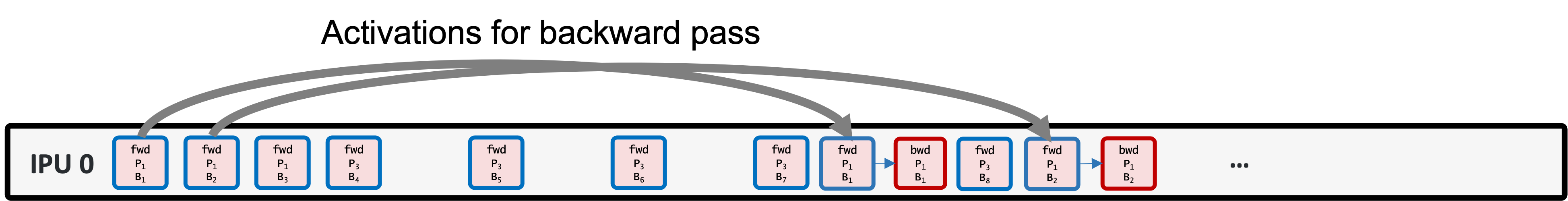
Fig. 5.1 Recomputation of activations increases the number of operations. Blue = forward, cyan=forward for recomputation, red=backward

In models that are memory intensive (and most deep-learning models are), using recomputation to save memory is more valuable than the extra execution cycles. For example, BERT Large would not fit in memory without recomputation (Fig. 5.2 and Fig. 5.3).

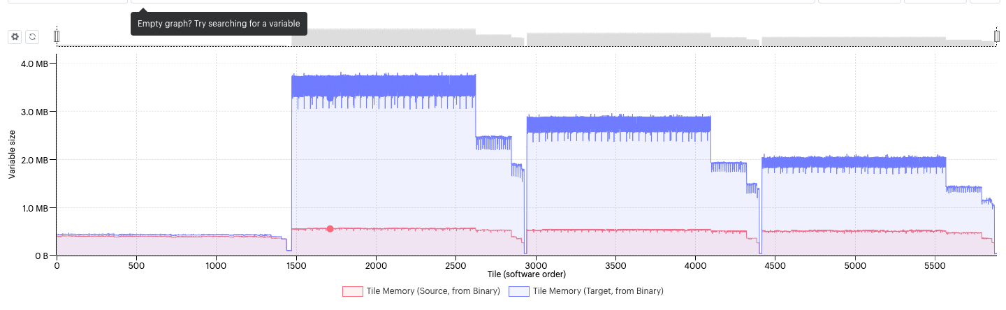
Fig. 5.2 Total memory use in a model without recomputation of activations (blue) and with recomputation (red).

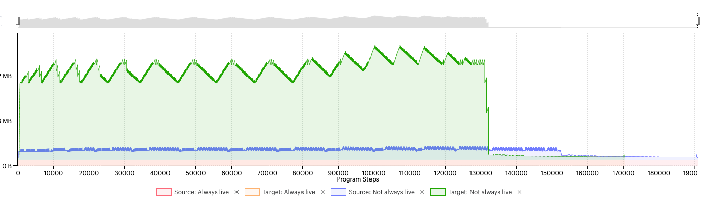
Fig. 5.3 The change in not-always-live memory for a model without recomputation (green) and for a model with recomputation (blue).

5.3.2. Recomputation checkpoints

Recomputation checkpoints are points in the computational graphs where all the activations are stored. Any activations in the graph from that point on will be recomputed from the previous checkpoint values, and stored in not-always-live memory, until the next checkpoint. Checkpoint positions in the graph can be set automatically by the frameworks or you can manually insert. When you pipeline a model, checkpoints are automatically inserted at the beginning of a pipelining stage.

The careful introduction of recomputation checkpoints, whether a model is pipelined or not, significantly saves always-live memory, since the amount of memory saved corresponds to all the activation FIFOs between two checkpoints.

The trade-off is an increase in compute cycles. Effectively, between two recomputation checkpoints, the backwards pass is replaced by a forward and a backwards pass. As a rule of thumb, the backwards pass takes between 2 to 2.2 times as many cycles as a forward pass.

In the inference mode, intermediate activations are never stored and hence recomputations are not required.

• In Tensorflow, recomputation can be enabled using the IPUConfig option allow_recompute. Different recomputation modes exist. The recomputation checkpoints can be set in multiple ways when using pipelining:

  • A tensor in the graph can be wrapped in a recomputation_checkpoint.

  • In Keras, a special layer is available to indicate the recomputation checkpoints:

  Keras recomputation checkpoints with Tensorflow 1.

  Keras recomputation checkpoints with Tensorflow 2.

• In PopTorch, recomputation is enabled by default when using a pipelined execution. Checkpoints can be added by wrapping one or more tensors in poptorch.recomputationCheckpoint.

  Note

  By default there is at least one checkpoint per pipeline stage.

• In PopART, you need to select a recomputation type first and enable it by setting the session option autoRecomputation. For instance:

  userOpts = popart.SessionOptions()
  userOpts.autoRecomputation = popart.RecomputationType.Standard
  

  When using the builder API, manual checkpoints can be added with the builder.checkpointOutput method. For instance, let’s define a simple graph and add a recomputation checkpoint to the output.

  # Set `RecomputeAll` to have all ops recomputed by default
  userOpts = popart.SessionOptions()
  userOpts.autoRecomputation = popart.RecomputationType.RecomputeAll
  
  def build_graph():
      builder = popart.Builder(opsets={"ai.onnx": 10, "ai.graphcore": 1})
      x_tensor = builder.addInputTensor(popart.TensorInfo("FLOAT", (1,)))
      y_tensor = builder.aiOnnx.mul([x, x])
      # Checkpoint y_tensor
      y_tensor = builder.checkpointOutput([y_tensor])[0]
      return y_tensor
  

  You can also force the recomputation of a specific output using builder.recomputeOutputInBackwardPass.

5.4. Variable offloading

The optimiser state parameters (for example, the first and second moments in ADAM) are always present in memory during training. You can also offload these to the host to save IPU memory. The optimiser states are only transferred once at the beginning (from host to IPU) and once at the end (from IPU to host) of the weight update step, so the communication penalty is much less than transferring model parameters.

Offloading variables to the host will create some exchange code, the size of which is difficult to estimate. It will also use temporary (not always live) data memory in order to store the input and output buffers from and to the host.

• In Tensorflow, variable offloading can be set with gradient accumulation and pipelining: TensorFlow 1, TensorFlow 2.

• In PopART it is possible to offload the optimiser state tensors in Streaming Memory using the tensor location setting.

• In PyTorch the same thing can be achieved by using PopTorch’s tensor location settings. To setup optimiser state offloading we can use setOptimizerLocation:

  opts = poptorch.Options()
  opts.TensorLocations.setOptimizerLocation(
     poptorch.TensorLocationSettings().useOnChipStorage(False))
  

5.5. Graph outlining

You can reuse identical code in different parts of the computational graph by outlining the code. This will keep only one copy of the code per tile and the graph will contain multiple call operations to execute the code. Without outlining, identical code at different vertices is always duplicated, taking up memory.

Note: You can think of outlining as the opposite of in-lined functions in C++.

In a Poplar graph, the mapping of the tensors to the vertices is static. When a section of code is outlined, the input and output tensors are statically mapped. This means that when the section of outlined code is called at different points of the computational graph, the input and outputs at this point of the computational graph must be copied into and out of the locations of the statically mapped tensors in the outlined code. The copy operations require more always-live memory and a penalty of using outlining is that you require more cycles.

We will illustrate how outlining works on an example using BERT transformer layers.

In the original, not outlined program, most of the code is under the top-level control program and there are only two additional functions (Fig. 5.4).

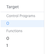
Fig. 5.4 Program tree in PopVision

Looking into the control program code we can see the self-attention blocks are repeated multiple times in the program tree (Fig. 5.5, Fig. 5.6). These self-attention blocks operate on large matrices and can take a large amount of program memory.

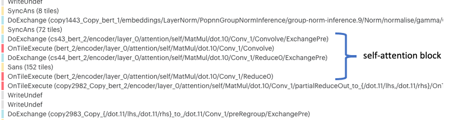
Fig. 5.5 First transformer layer

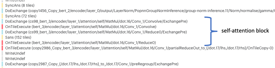
Fig. 5.6 Second transformer layer

And similarly for the 22 remaining layers of BERT Large. The code, required for this self-attention operation, is thus duplicated many times and this increases the total code memory use.

When the self-attention block is outlined, the outlined section of code is now an independent Poplar function. Looking at the control program, we can see the self-attention blocks of code have been replaced by a call to a Poplar function (Fig. 5.7, Fig. 5.8).

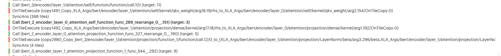
Fig. 5.7 First transformer layer with outlining

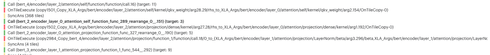
Fig. 5.8 Second transformer layer with outlining

The “target” argument is the identifier of the Poplar function being called. So, in this case, Function 3 is being called. Looking into Function 3, called from Call(target: 3) we see the self-attention block (Fig. 5.9).

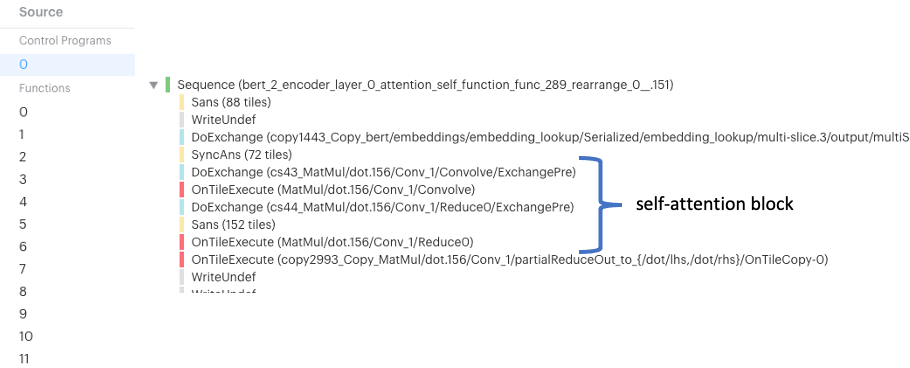
Fig. 5.9 Details of self-attention block after outlining

The function exists only once in memory and is re-used for multiple input and output tensors. Poplar adds copy operations in the graph so that different variables (tensors) can be used as inputs to the single function. The developer could expect the function to use pointers to eliminate the need for copies, however this is not possible in the static graph model of Poplar, so outlining saves always-live code memory but adds copies at run time.

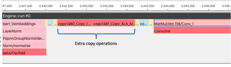
Fig. 5.10 Execution graph (from PopVision) with outlining

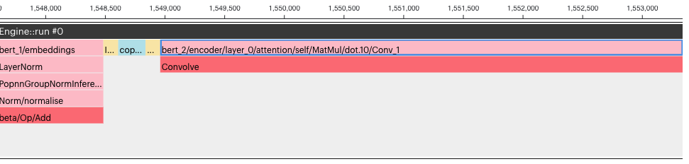
Fig. 5.11 Execution graph (from PopVision) without outlining

The self-attention block spans many execution cycles (in Fig. 5.10 only the start of the self-attention block is shown). So, the execution cycles added for the extra copy operations for the outlined code do not increase the total execution cycles by too much.

Outlining is performed by default by PopART and Tensorflow. They both give the user different levels of control:

• Tensorflow provides a decorator to define outlined functions. Also, optimizations.enable_graph_outlining can be set in IPUConfig to enable/disable outlining.

• In PopART the session options give access to enableOutlining to enable/disable it. outlineThreshold controls the threshold after which subgraphs should be outlined. Low values result in more sub-graphs being outlined.

5.6. Reducing the batch size

In some applications, it may be possible to use a smaller batch size to reduce memory requirements.

If you reduce the global batch size (that is, the total number of samples processed between weight updates) for training, you should also reduce the learning rate. Scaling the learning rate by the same factor as the batch size has been found to be effective - see §2.1 of Accurate, Large Minibatch SGD: Training ImageNet in 1 Hour by Priya Goyal et al. for details.

Using a smaller micro-batch size won’t necessarily hurt performance. The IPU’s architecture makes it better for fine-grained parallelism than other processors which enables better performance at low batch sizes. Further, researchers at Graphcore have shown that smaller batch sizes can stabilise training. See Revisiting Small Batch Training for Deep Neural Networks by Masters and Luschi for full details.

However, there are some operations, such as batch normalisation, that are calculated across a mini-batch. The performance of these operations can degrade when reducing the batch size. If this causes problems, you may choose to replace batch normalisation with group, layer or instance normalisation instead.

As an alternative solution, you may choose to use proxy normalisation, a technique developed by researchers at Graphcore. Proxy normalisation is designed to preserve the desirable properties of batch normalisation while operating independently of the batch size. A TensorFlow 1 implementation is available in Graphcore’s public examples. Proxy normalisation was first described in the paper “Proxy-Normalizing Activations to Match Batch Normalization while Removing Batch Dependence” by Labatie et al.

Note

From Poplar SDK 3.1, TensorFlow 1 will only be supported in CentOS 7. In addition, Examples and Tutorials for TensorFlow 1 are only available up to version 3.0 of the SDK. There has been limited testing of the 3.0 versions of the TensorFlow 1 tutorials and examples with Poplar SDK 3.1.

5.7. Writing a custom operation

If you have a particular operation in your model that is using a lot of memory, you may find it useful to write a custom operation using a lower-level library that uses less memory.

Refer to the technical note “Creating Custom Operations for the IPU” for details and links to additional resources on writing custom operations.