3. Mapping a model to an IPU system
This section describes how to map a model to the Graphcore IPU hardware and the Poplar graph programming framework.
At this stage, we are not considering any optimisation that could improve the data memory use, such as recomputation or offloading. We are simply interested in assessing how large the model is and how many IPUs may be required to make it fit.
This section describes:
How a machine learning algorithm is mapped onto a Poplar graph
How Poplar uses IPU memory at runtime
How to estimate the memory use of the model tensors at the design stage
3.1. Computational graph of ML model training
Most deep learning models are trained using backpropagation and can be represented by a computational graph similar to that in Fig. 3.1.
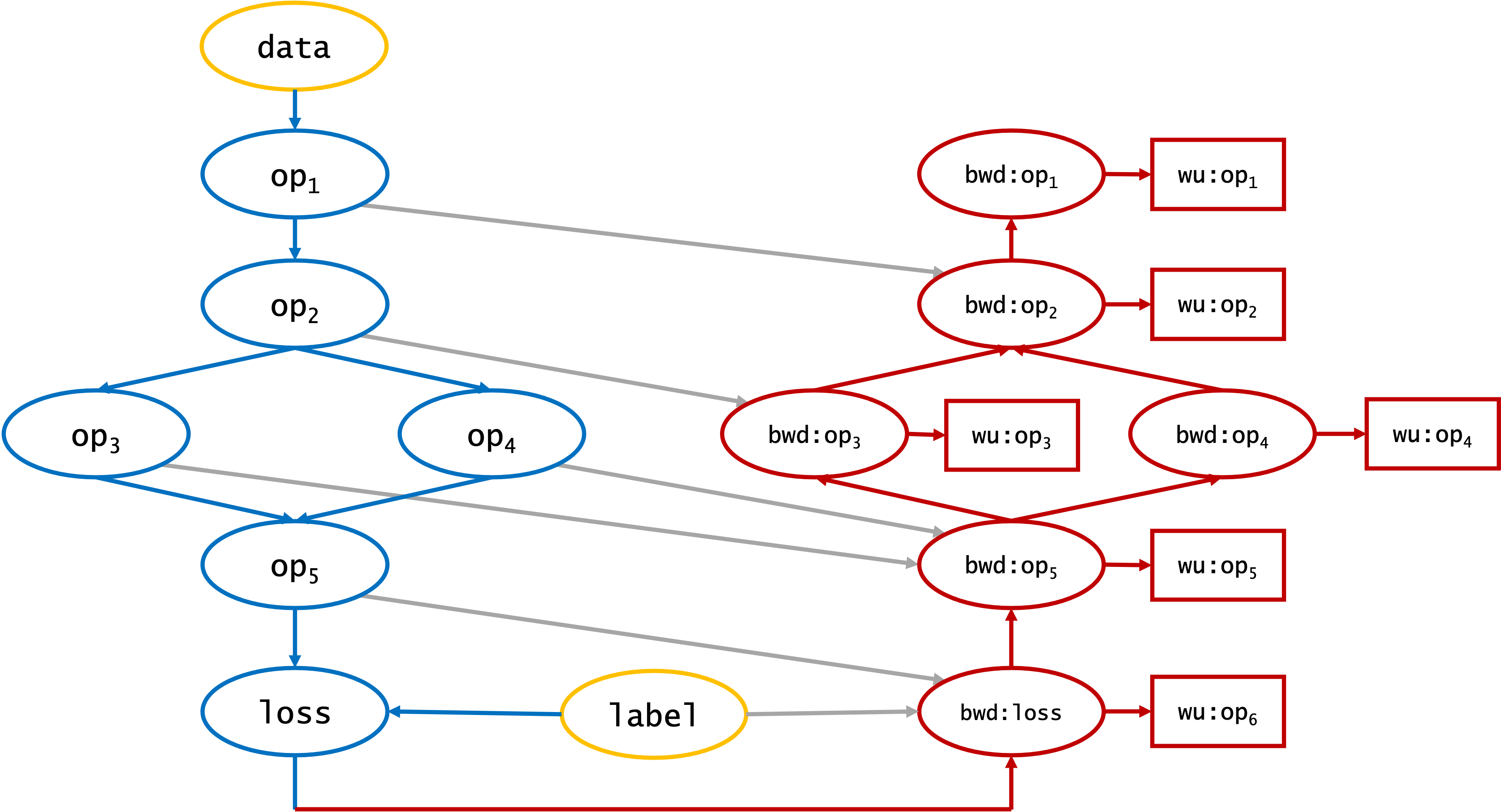
Fig. 3.1 Computational graph of training a simple network using backpropagation. op is a forward-pass operation, bwd: the corresponding backward pass operation and wu: the weight update operation.
The mapping of the computational graph onto the IPUs is left to the AI engineer and is critical for achieving performance targets. Note that this exercise may be constrained by the capabilities of a given ML framework. For example, PopART offers more flexibility with partitioning the graph into low-level operations than high-level frameworks such as TensorFlow or PyTorch.
3.2. Understanding the memory mapping of a computational graph
The Poplar compiler takes the computational graph and creates an executable for running on IPU systems. The IPU memory used by the computational graph is allocated when Poplar compiles the graph. This memory is composed of:
code (for example, linear algebra operations)
input and output tensors
code and buffers supporting data exchanges
3.2.1. Machine-learning models use of memory
Before porting a model to an IPU system, it can sometimes be beneficial to estimate the total memory required by a given machine learning model. The total memory required can be decomposed into:
Data and variables of the model such as
trainable parameters (for example, weights and biases)
non-trainable parameters (for example, the mean and variance statistics of the local batch in the normalisation layers)
activations (outputs of a layer)
optimiser state variables (for example, the first two moments in the Adam optimisers)
gradients with respect to the weights
Program code required to calculate:
the model output during inference or during the forward pass
the losses and gradients during the backward pass
the weight updates, which depend on the optimiser used
In addition to data and program code, Poplar also allocates memory to store the code and data buffers used during the exchange phase. This memory is used during communication between different entities, such as compute sets, tiles and IPUs.
3.2.2. IPU memory used by a Poplar computational graph
The memory used by a Poplar graph is composed of:
Tensor variables, which contain the data at the input and output of a vertex, such as weights, optimiser states, and weight update values;
Vertex code, which is generally the code performing numerical operations;
Vertex state memory, used by variables local to a vertex instance;
Exchange code, which contains the code needed during the exchange phase
Exchange buffers, which contain data used during the exchange phase.
The exchange code and buffers exist for three types of exchanges:
Internal exchange for exchanges between tiles on a same IPU
Inter-IPU (or global) exchange for exchanges between IPUs
Host exchange for exchanges between the IPUs and the host
First-in first-out (FIFO) queues on the IPU also exist to enqueue and dequeue data coming from the host.
3.3. Always-live and not-always-live memory
The memory used by the data is allocated by the Poplar compiler at compile time. The compiler tries to re-use memory by considering memory use over the entire duration of the graph execution. For example, two variables may share the same memory addresses if the lifetime of each variable does not overlap.
Memory that is allocated to a specific entity (for example, compute set code, variables and constants) for the entire lifetime of the graph execution is called always-live memory.
Similarly, the data for not always live variables are only needed for some program steps. If two variables are not live at the same time, they can be allocated to the same location, thus saving memory. This memory is referred to as not-always-live memory.
It is the combination of always-live and not-always-live memory requirements for a model that determine the total memory use and therefore affect performance.
3.4. Tensor variables memory use
3.4.1. Number of model parameters
At this stage, it is worth doing some back-of-the-envelope calculations to identify which elements of the models (such as convolution kernels, dense layers, embedding tables) may be the largest contributors to the data memory use.
The size of these blocks can be related to some model hyperparameters, such as sequence lengths, image size, number of channels, embeddings table size, and hidden representation size.
Layer |
Inputs |
Number of parameters |
|---|---|---|
Convolution layer |
Kernel size \((h,w)\), \(N\) filters, \(C\) channels |
\((w \cdot h \cdot C + 1) N\) parameters (weights and biases). |
Dense layer |
Input size \(n\), output size \(p\) |
\(n \cdot p\) weights and \(p\) biases. |
Batch norm |
Tensor size \(n\) on normalisation axis (In a convolution layer, normalisation is done along the filters.) |
\(2n\) moving average parameters (training and inference) plus \(2n\) scale and location parameters (\(\beta\) and \(\gamma\) training only) |
Layer norm |
Input length \(n\) |
\(2n\) parameters |
Embeddings table |
Vocabulary size \(N\), hidden size \(h\) |
\(N \cdot h\) parameters |
Note that normalisation layers contain parameters that are “non-trainable”. Typically, during training, these are based on the statistics of a micro-batch, and during inference these are re-used from the training stage. These always reside in memory but there will be no optimisation parameters associated with them.
3.4.2. Number of activations
During inference, the outputs of the activation functions (referred to as activations) do not need to be stored long-term, as they are typically only used as inputs to the next layer. Note: this is not always the case and some models, in particular image segmentation models, need to pass the activations between multiple layers during inference. If these layers reside on different IPUs, the activations will need to be stored and exchanged, generally increasing both data, code and exchange memory requirements.
The memory use of activations during training is considered in the following sections.
3.4.3. Number of optimiser states (training only)
During training, the weight update step of the optimiser may rely on state variables. For example, the Adam and LAMB optimisers need to store the first (\(m\)) and second (\(v\)) moments between weight updates. These optimiser states will need to be stored in always-live memory and scale linearly with the number of trainable parameters in the model.
3.4.4. Number of backpropagation variables (training only)
During training via backpropagation, you need to make the activations available in the backward pass in order to calculate the gradients with respect to the activations and weights. As a first approximation, we should consider that all the activations are stored in always-live memory, although in practice recomputation of activations (detailed in Section 5.3, Activation recomputations) is often used.
The number of activations required (either for storage or computation) scales linearly with the compute batch size.
The gradients (with respect to the weights) also need to be stored during training. The parameters of every trainable model have associated gradients, and these need to be stored in memory.
Therefore, the memory needed increases by:
\(N_{gradients} = N_{activations} \times B_{size}\)
\(N_{backprop\_ vars} = N_{weights} + N_{biases} + N_{non\_ trainable} + N_{optimiser\_ states}\)
where \(N_{gradients}\) is the number of gradients, \(N_{activations}\) is the number of activations, \(B_{size}\) is the compute batch size, \(N_{backprop\_ vars}\) is the number of backpropagation variables, \(N_{weights}\) is the number of weights, \(N_{biases}\) is the number of biases, \(N_{non\_ trainable}\) is the number of non-trainable parameters and \(N_{optimiser\_ states}\) is the number of optimiser states.
3.4.5. Determine total memory used by variables
The total amount of memory required for all the model parameters is thus:
In inference: \((N_{weights} + N_{biases} + N_{non\_ trainable}) \times N_{FP}\)
In training: \((N_{weights} + N_{biases} + N_{gradients} + N_{optimiser\_ states} + N_{backprop\_ vars}) \times N_{FP}\)
where \(N_{weights}\) is the number of weights, \(N_{biases}\) is the number of biases, \(N_{non\_ trainable}\) is the number of non-trainable parameters, \(N_{gradients}\) is the number of gradients, \(N_{optimiser\_ states}\) is the number of optimiser states, \(N_{backprop\_ vars}\) is the number of variables required to store the gradients with respect to the weights during backpropagations and \(N_{FP}\) is the number of bytes used by each variable and depends on the numerical precision (half or single) chosen.
3.5. Vertex code and exchange memory use
Accurate estimation of the exchange code size is very difficult, if not impossible, at the design stage of a model. The internal exchange code is statically compiled, so dynamic access to tensors is not well optimised. It is safer to consider that the entire tensor will be allocated instead of slices of tensors.
The exchange code is always-live in memory.
Predicting the memory used by the exchange code and vertex code is dependent on the model and on the Poplar compiler optimisations. There is no general approach to determine this memory use. The best way to estimate the proportion of the memory used by the vertex code and exchange is to start with a small model and vary parameters such as micro-batch size, number of hidden layers and number of replicas. This will give an estimate of how the memory use grows with the model size and the proportion of the memory used for code versus data (Section 3.4, Tensor variables memory use).
Some rules of thumb to minimise the exchange code size are:
Lots of small tensors are less efficient than fewer large ones.
The tensor layouts may matter, since the tensors may need to be “re-arranged” during the exchange, which increases the temporary memory use.