7. Scaling an application over multiple replicas
Training a machine learning model can require an enormous amount of data. This amount of data makes training time consuming. To speed up the process, one solution is to have many replicas (copies) of the model. The learning data can then be split across these replicas, which are placed on multiple IPUs (horizontal scaling).
While scaling applications horizontally can speed up training, there can be a variety of reasons for scaling to behave unexpectedly and a thorough analysis is required. This section discusses techniques for performance improvement when using data-parallel processing over multiple replicas.
The number of IPUs occupied by the model is always a power of 2 due to the required ring structure for communication. When doubling the number of IPUs for your model in a data-parallel processing scheme, the ideal behaviour is a doubling of the training or inference throughput and halving the time to train. Several techniques can be applied to get as close as possible to this.
For more details about the architecture of the scale-out IPU hardware, refer to Section 7.9.1, Scale-out IPU hardware architecture.
7.1. Quick guide to scaling
If your scaled application does not compile, refer to Section 5, Common memory optimisations. If your throughput does not scale, good first steps to try are using the PopDist tools to optimize host I/O (Section 4.3.2, Multiple SDK instances and replication: PopDist) or changing the gradient accumulation (Section 4.3.1, Graph replication) to reduce communication between IPUs. If these standard techniques do not help, continue reading to discover background knowledge, analysis tools, and several other techniques to boost performance.
7.2. Analyse your scaling behaviour
To improve scaling, you first must measure the throughput and then drill down into what is affecting it. What is especially critical is to figure out which parts of the application code need constant time and thus will not scale (Amdahl’s law). In some cases, those can be parallelized to benefit from scaling. In other cases, they can be moved into the pre- or post-processing stage, for example importing all libraries at the beginning or uploading final reports to Weights & Biases (Weights and Biases is a widely-used library for performance metric logging and exploration in machine learning). There are however some situations when they cannot be avoided, and you should go through the calculation, as described below, to determine if they are the sole reason for reduced scaling performance. It is important to remember that any parts of the application that do not scale with the number of concurrent processes will be a performance bottleneck and an upper bound of the maximum throughput achievable.
With 1/throughput, you can get a rough estimate of how much of the total processing time is for a single sample. This number is not the latency but sometimes can be helpful.
You can also measure latency. Use the PopVision tools for a better drill down.
The PopVision System Analyser can provide a detailed overview of the time used by the different components of an application (initialization, weight loading, data communications, different layers, gradient communication, gradient update, etc.). Sometimes, the PopVision Graph Analyser can be helpful too. It shows data about the graph program, memory use, and the time spent on code execution and communication. This is useful when changing from one to two replicas or when going across Pods. Note that you can also add your own time measurements to the code and even integrate them into the System Analyser. More information can be found in the tutorial about instrumentation, in the System Analyser user guide and in the PopVision Trace Instrumentation Library documentation, which contains examples in Python. For large applications, with distinct phases, it is helpful to get a separate profile for each phase. For example, for an application such as ResNet-50, there is an initialization phase that includes compiling the graph and loading it onto the IPUs, multiple training phases, phases in between training phases where checkpoints get stored, a graph swapping phase for the validation, and the final validation phase.
What can help is to measure the time distribution and then after doubling the number of replicas/IPUs, check which components double their compute, which is the ideal outcome, and which components are not impacted at all by the increased compute.
7.2.1. Estimating the theoretical throughput
There are several assumptions that can be made about the system that will allow you to estimate the theoretical throughput of the application.
Usually, the training is parallelised across R replicas, each working on different training samples. If we assume that one replica fits on one IPU, as in TensorFlow 1 ResNet-50, then on a Pod16, there are 16 replicas (R=16). Similarly, on a Pod128 there are 128 replicas (R=128).
The training consists of two phases. The first phase happens when a replica processes a batch. In the second phase, all the replicas share their gradients, using an allreduce (Section 7.9.2, GCL allreduce), and then update the optimizer state.
The number of batches processed before the gradients are reduced is specified by the gradient accumulation factor. This factor depends on the machine and is usually a fixed parameter for a particular model. Gradient accumulation is described in detail the IPU Programmer’s Guide.
When using replication and gradient accumulation, the number of samples processed by one forward or backward pass in a single replica is defined to be a micro batch (see definition of micro batch in IPU Programmer’s Guide). The batch size used for a weight update is then:
micro batch
size * gradient accumulation factor * number of replicas
.
For distributed batch normalisation, which then occurs at the micro batch level, the batch processing also involves cross-replica communication. Replicas are clustered into groups and the parameter controlling the number of IPUs per group is called the span. For many models, we use a span of 2. For each layer, and for each pass (forward and backward) each group does an allreduce.
Because of the steps described above, with \(T_{MB}\) being the time needed to process a micro batch, \(T_{AR}\) being the time to perform an allreduce on the gradients (and update the optimiser state), the time for one replica to process \(GA * MBS\) dataset elements (\(T_{GA * MBS}\)) can be written as:
where \(GA\) is the gradient accumulation factor and \(MBS\) is the micro batch size.
Therefore, the number of dataset elements processed per second, by all the replicas, can be written as:
Having this model helps in two ways. First, it sets a baseline to which we can compare actual results and detect abnormal performance. Second, we can use it to extrapolate the effect an optimisation will have on the overall throughput. On a single Pod, the time to do an allreduce is the time taken to send the tensor being reduced from one replica to another over the links, twice (this ignores the syncing and latency costs). See Section 7.9.2.1, GCL allreduce on a single POD for more details.
On multiple Pods, apart from doing the allreduce within each IPU-Link domain (and thus having the same time cost as for a single Pod), there is also a reduction happening over the GW-Links. During such a reduction only 1/R of the data is reduced between two given replicas (for two Pods). See Section 7.9.2.2, GCL allreduce with many Pods for more details.
7.3. Constant or slowed-down processes (Amdahl’s law)
Amdahl’s law describes how much accelerating a component will benefit in overall speed-up depending on how much this component is actually used in the overall processing. For example, if 50% of your processing is constant (for example, limited by the host or host-IPU communication), by quadrupling the compute for the non-constant part, you will not get the desired speed-up of 4x but instead you could get 2.5x, or 62.5% scaling efficiency. So, after the analysis of the scaling behaviour and determining the parts that do not scale well (especially because they require constant processing time), tackling these is usually the road to success.
Running a program on an IPU can be separated into four components in a very simplified perspective: host processing, IPU to host communication, IPU processing, and communication between IPUs. The three key locations are host memory, Streaming Memory, and In-Processor Memory. Prefetching is a way of overlapping transfer (of code and data) between the host memory and Streaming Memory during IPU-to-host communication. I/O tiles on the IPU allow for overlapping the transfer of data between Streaming Memory and In-Processor memory during communication between IPUs.
When scaling the processing by adding more IPUs, the on-device IPU processing usually scales perfectly. However, depending on the application, the other parts such as communication and host processing could be at the limit of their capacity and become bottlenecks because they cannot handle the increased influx of data. The host might be able to prepare enough data for one IPU without impacting the throughput because processing happens concurrently. However, with more IPUs added, the host might be saturated and be unable to send data to the IPUs fast enough to avoid leaving them idle.
One way to improve scaling is to add more hosts to scale the pre-processing. Other ways are to apply software engineering techniques such as parallelizing implementations, overlapping different computations, or improving code efficiency such that the constant time is reduced to a minimum. Sometimes, there is also a solution from the application point of view by running the constant parts only in a warm-up or cool down phase (for example, imports or report uploading, respectively) or reducing the number of occurrences (for example, instead of storing a checkpoint every 0.1 epochs, it might be sufficient to store it only every epoch or even less).
For communication betweem IPUs, it is better to merge results of different
data types and lengths, and communicate all these together. For example,
if your code has many allreduce operations, it is better to merge them.
TensorFlow has maximum_reduce_many_buffer_size in the IPU configuration that defines the maximum size a cluster of reduce operations can reach before it is scheduled for transfer.
7.4. Graph compilation and executable loading
While running an application, sometimes graphs might be compiled and
swapped, for example, to switch between training and validation.
However, the graphs can be pre-compiled even before running the program
and the respective executables stored on permanent storage to be accessible for any
follow up execution without impacting the throughput. Additionally, by storing the weights of interest in checkpoint files,
validation can be implemented separately at the end of a run, such that
the executable gets swapped only once. Alternatively, with potentially
some more engineering effort, it is possible to run training and
validation with the same graph by suppressing the training update. You
can achieve this, for example, by suppressing a gradient update by
setting the learning rate, weight decay, and other update weights to
zero. You can also adjust the validation batch with padded samples, if
it has a fixed size that is not divisible by the global batch size. Note
that the IPU can handle branching conditions. Hence, it is possible to
switch between distinct parts of the computational graph with something
as simple as a tf.cond in TensorFlow and, for example, using the learning
rate or a dedicated variable to switch between training and validation.
7.5. Host-I/O optimisation
When scaling from 1 to 16 IPUs without further adjustment, most of the time only one host machine is used with a single Unix process. If we consider the most extreme case of 100% occupation of host processing or bandwidth when running with 1 IPU, any increase in the number of IPUs will result in no improvement of speed or may even reduce the speed due to conflicting processes.
The key ingredients for host-I/O optimizations are the PopDist library
and the PopRun command line utility (Section 4.3.2, Multiple SDK instances and replication: PopDist).
You can see PopRun as a replacement for mpirun that is specifically
designed for the IPU. It supports distributing the data preparation and
data loading over multiple hosts to support large numbers of IPUs,
including the bridging of multiple Pods. PopRun allows you to run
multiple instances of your model (typically a Python process), that
can be distributed over multiple host machines connected to the same
Pod.
For many tasks, the data coming out of the model such as model prediction, metrics, and losses, requires significantly less bandwidth than the data going into the model (input data). A notable exception is image segmentation.
One common question when analysing scale-out performance is whether the host can feed data fast enough to the IPUs, or whether the Host-IPU bandwidth is creating a bottleneck.
An approach that can be used to profile host I/O communication is to analyse the following three cases:
Real data provided by the host: Several applications come with dataset benchmarks that could be used to analyse the data loading. In TensorFlow, we also provide some APIs you can use for testing.
“Generated” data provided by the host: This means some data is generated on the host with minimum pre-processing, to avoid increasing the host CPU load. Typically, random data is generated.
“Synthetic” data generated directly on the IPU: This is controlled by different options in the ML frameworks. For the data to be representative, additional options are provided, for example, you can create random data on the IPU with:
the
--use_synthetic_dataPoplar flags variable in TensorFlow 1 and TensorFlow 2,the
enableSyntheticDataoption in PyTorch,the
syntheticDataModein PopART.
Throughput with synthetic data is always expected to be better than with real or generated data. However, if this difference in throughput changes significantly when the number of replicas is increased, host-I/O optimizations are necessary as explained in Section 4.3.2, Multiple SDK instances and replication: PopDist.
A simple way to check the host CPU and memory workloads is to run top or
htop in a separate terminal. These commands display a complete list of all
processes that are running. You can then use lcpu to get stats about the
host CPU. Host processing can be impacted by the type of processor, the number
of cores and the number of NUMA nodes. For example, when using PopRun to scale your application, the number of PopRun
instances should be less than or equal to the number of NUMA nodes. This way,
there is no interference on the compute and memory resources between the
independent processes so they will not slow each other down. Apart from
caching or precomputing the host part, Graphcore’s disaggregated host
architecture allows more than one host to be used, to scale the host processing as needed.
For example, for scaling ResNet-50 to a Pod64, we needed four hosts
with eight separate instances to load and pre-process the data, whereas BERT
needed only a single host. For scaling applications across Pods, you must use
PopRun with at least one host per Pod. NUMA awareness can be crucial for
performance and can be easily set up with PopRun.
If data cannot be loaded fast enough because it is on a slow network drive or multiple people are accessing it, copying the data to a faster drive and caching it during the processing can result in speed-ups.
If a model has a low computational workload compared to the size of the data it processes, it can also be helpful to increase the model size and complexity.
Before you start with host-I/O optimisations, make sure that the data you want to transfer actually needs to be transferred. Sometimes, input data can be transferred in lower resolution (8-bit integer format for images, for example) or even generated on the IPU, for example when sampling random data in simulations. Instead of transferring predictions it is usually much more efficient to transfer derived data such as aggregated metrics instead.
7.6. Batch size and gradient accumulation count
A simple scaling approach is to accept doubling the batch size when doubling the number of replicas. However, from a machine learning and parameter optimization point of view, this might not be desirable since larger batches might decrease convergence speed. Note that by not scaling the batch size, it is expected that throughput drops to some degree because either the IPU has less workload and/or there are more frequent gradient updates and communications. Hence, it is good to look at this point separately. Sometimes, scaling performance can be simply improved by aggregating gradients a bit longer before triggering an update. This concept is called gradient accumulation. For more information on gradient accumulation, refer to the following sections in the framework user guides:
There are also more modern machine learning approaches to avoid the overhead of gradient communication, for example as described in Parallel Training of Deep Networks with Local Updates.
7.7. Memory optimization for more replicas
When switching from training a model on one IPU to multiple IPUs, gradients must be aggregated across the IPUs, incurring a communication overhead that increases with the number of replicas. Additionally, the communication of gradients requires additional exchange code since code and data reside on the IPUs. The increase in exchange code size when scaling might cause the model to run out of memory.
The respective sizes can be analysed by comparing the different processing profiles with the PopVision Graph Analyser.
A simple approach would be to reduce the batch size to get the model to fit in memory. However, by reducing the batch size, you usually reduce the utilization of the IPU since it will now process less data in one run. So, this will also reduce your scaling. One approach to reducing the memory for code is to fine-tune the available memory proportion.
And there are a few other tools to save memory as described in Section 5, Common memory optimisations. This way, you might be able to keep the batch size and hardware utilization the same.
The Graphcore Communication Library (GCL) exposes the syncful.useOptimisedLayout option. This option can be
controlled with the GCL_OPTIONS environment variable and takes a Boolean
value). The default is true, which optimizes GCL code paths for memory,
but if memory pressure is not a problem, you can use false which might reduce the cycle count at the cost of higher memory usage. OptionFlags contains more information on the syncful.useOptimisedLayout option.
7.8. Pipeline optimization and replicated tensor sharding
There are a few other tools that can be used in some application settings. For example, a model that runs on a single IPU (using recomputation) might be faster when using two IPUs in a pipeline setup instead of using replication. Changing the pipeline setup can also help in the context of replicated tensor sharding where optimizer states or other variables are distributed across multiple replicas instead of having multiple copies. With more replicas, this feature can be potentially applied.
7.9. Technical background
This technical background section gives more details about the scale-out IPU hardware architecture and about the GCL implementation of allreduce.
7.9.1. Scale-out IPU hardware architecture
To understand how the Pod system scales, it is useful to understand how it is built in the first place and what building blocks are used.
The first building block is an IPU (Fig. 7.1). The IPU has two edges: the west edge and the east edge. On these edges there are link controllers and a PCIe link (Host-Link) to the host. A link controller is a customised PCIe port and a Graphcore-specific PCIe cable (an IPU-Link cable) can be plugged between two link controllers on different IPUs. In this way the IPU-Links are used to make direct connections between individual IPUs.
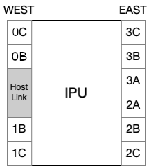
Fig. 7.1 A view of IPU connectors
The second building block is an IPU-Machine (Fig. 7.2), which is a blade consisting of four IPUs and an IPU-Gateway chip. The four IPUs in an IPU-Machine are connected to form a rectangle and are numbered row first, starting from bottom left. IPUs 0 and 1 and IPUs 2 and 3 are connected via IPU-Links on their east edge link controllers (2A, 2B, 2C, 3A, 3B, 3C). Additionally, IPUs 0 and 2 and IPUs 1 and 3 are connected via IPU-Links on their west edges. The connection between IPUs 0 and 2 uses the 0C and 0B link controllers, whereas the connection between IPUs 1 and 3 uses the 1B and 1C link controllers. This leaves two link controllers unused on each IPU: 1B and 1C on IPUs 0 and 2; 0B and 0C on IPUs 1 and 3. These unused link controllers are used when connecting IPU-Machines together and become GW-Links. The connections are shown in Fig. 7.2.
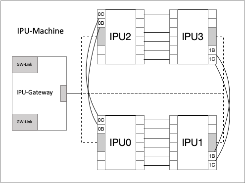
Fig. 7.2 A simplified view of an IPU-Machine.
The IPUs are also connected to the IPU-Gateway via their Host-Link. The IPU-Gateway acts as a “host” for all four IPUs on an IPU-Machine. It also provides access to the GW-Link connections.
The next building block is a Pod. IPU-Machines, each containing four IPUs, are scaled vertically to form a Pod system. These can vary in size, for example there are four IPU-Machines in an IPU‑POD16 or a Bow Pod16 and 16 IPU-Machines in an IPU‑POD64 or a Bow Pod64. A Pod64 is the standard building block for scale-out. The IPU-Machines in a single Pod are connected using IPU-Links to form a 2D vertical torus or a mesh topology. Apart from IPU-Link connections, there are also Sync-Links for sending sync signals which topologically follow the IPU-Link connections. Two IPU-Links from each IPU in an IPU-Machine go to external connectors so they can be connected to other IPU-Machines. The links provide a bandwidth between IPUs of 64 GB/s (bidirectional).
IPUs in a Pod (Fig. 7.3) are numbered following the same pattern as in the IPU-Machine (Fig. 7.2), starting with the lowest IPU-Machine in the Pod. The bottom left IPU in the lowest IPU-Machine is IPU0. The one to its right is IPU1. The remaining two IPUs on the same IPU-Machine are IPU2 and IPU3, followed by IPU4 to IPU7 on the next IPU-Machine and so on, all the way up to IPU62 and IPU63 on the top-most IPU-Machine.
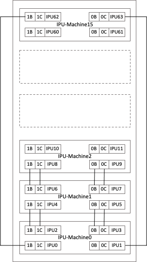
Fig. 7.3 A schematic of an IPU‑POD64. The top views of the IPU-Machines (IPU-M0 to IPU-M15) are depicted. IPU-Machines are installed such that IPU0 and IPU1 are towards the front of the Pod.
Fig. 7.4 shows the mapping between the external ports on the front panel of the IPU-Machine and the internal ports.
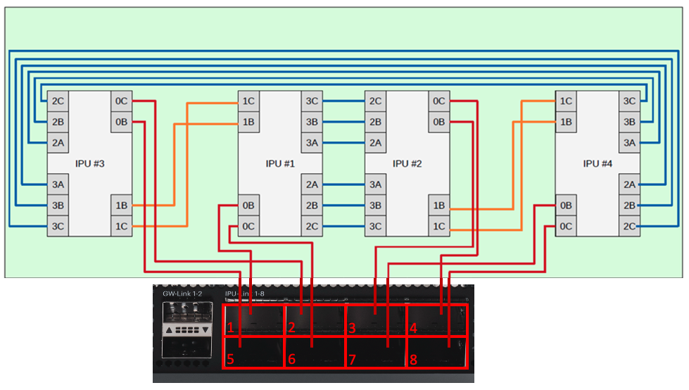
Fig. 7.4 IPU connections within an IPU-Machine and how it maps to the external ports on the IPU-Machine front panel
The last building block is a cluster of Pods (Fig. 7.5).
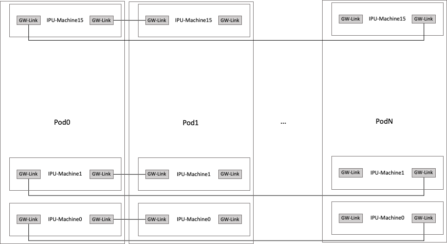
Fig. 7.5 A cluster of Pods
Pods can be scaled horizontally using GW-Link cables to connect IPU-Machines in adjacent Pods together. GW-Links use 100 Gb Ethernet (100 GbE) and are connected to form a logical torus topology in the horizontal dimension, thus providing an aggregated bandwidth of 200 GBps between a pair of IPU-Machines.
When working with multiple Pods, we introduce the concept of an IPU-Link domain, which is a set of IPUs in a cluster that are connected solely using IPU-Links. An IPU-Link domain can be all of the IPUs in a Pod, or some subset of them. A Pod64 is the largest single IPU-Link domain Pod system.
Connections between Pods are such that an IPU-Machine in a Pod in the middle of the cluster is connected to the IPU-Machines installed in the same slots on neighbouring Pods (Fig. 7.5). For example, IPU-M0 in a Pod is connected to the IPU-M0s on both neighbouring Pods. The leftmost and rightmost Pods are also connected, forming a ring. These IPU-Gateway to IPU-Gateway connections using GW-Link cables are usually not direct. Instead, the GW-Links are connected to a switch, which then implements the required connectivity.
A single Poplar host can be connected to a single IPU-Machine and communicates with all replicas. Alternatively, multiple hosts can be attached to multiple IPU-Machines, each machine addressing a partition of all replicas. Each host to IPU-Machine connection is based on 100 GbE.
There are two distinct allreduce implementations that depend on the underlying physical topology. In the description that follows, NxMs stand for the physical size of the topology, with N being the vertical size and M being the horizontal size:
All traffic over IPU-Links, unless otherwise stated, is bi-directional. This enables implementation of a single pass allreduce. By default, the IPU-Links are logically connected in a 2xN mesh topology (sometimes called a ladder) but they may also be connected in a 2xN torus topology (wheel) or a 2x2xN torus topology (Barley-twist)
The NxM 2D torus is connected with IPU-Links as a torus in the first dimension and GW-Links in the second dimension. NxM usually represents the number of IPU-Link Domains. For example, if you have two physical Pod64s, you can subdivide each of them into 4xPod16 connected with GW-Links. In this case M=8. So, the topology would be 8xPod16or given the NxM notation, 16x8.
The allreduce operation is performed here as a multi-phase operation:
Do a reduce-scatter of the data in the first dimension using the IPU-Links. Each IPU now holds a (1/N) part of the resulting sub-vector.
Do an allreduce in the second dimension of all sub-vectors using the GW-Links - with each of the N parallel allreduce operations processing (1/N) of the original size.
Do an allgather in the first dimension using the IPU-Links to distribute the data to all IPUs.
7.9.2. GCL allreduce
When doing data-parallel learning, there are many replicas, each working on their own data in parallel. At regular points, replicas share with each other what they have learned locally. The operation used for this is the allreduce. At the beginning of the allreduce operation, each replica has a tensor of local values. At the end, each replica has a tensor containing the elementwise result of the operation performed on all the replica local tensors.
For example, with two replicas each having an input with four elements:
Start values:
Replica0: {1, 2, 3, 4}
Replica1: {10, 20, 30, 40}
End values:
Replica0: {11, 22, 33, 44}
Replica1: {11, 22, 33, 44}
The Graphcore Communication Library is designed to support ML workloads at scale for IPU-based machines and it efficiently supports IPU to IPU communications for topologies formed by IPU-Machines interconnected to form Pods. GCL consumes a replicated Poplar graph and a Poplar program to which it adds vertices, tensors and CrossReplicaCopies, amongst other things. GCL contains an allreduce implementation.
7.9.2.1. GCL allreduce on a single POD
When there is only one Pod, the algorithm used by GCL is the ring reduce. Ring reduce has two phases: a reduce scatter and an allgather. It requires replicas to communicate with their neighbours only.
At the beginning of a reduce scatter, each of the R replicas has a tensor of local values with T elements. At the end, each replica has a tensor with T/R elements. This result tensor contains the elementwise sum of all the replicas’ local tensors. The reduce scatter has R-1 steps. At each step, each replica sends and receives T/R elements.
For example, with two replicas each having an input with four elements:
Start values:
Replica0: {1, 2, 3, 4}
Replica1: {10, 20, 30, 40}
End values:
Replica0: {11, 22}
Replica1: {33, 44}
The allgather operation picks up where the reduce scatter stopped: each of the R replicas has a tensor with T/R elements, containing the sum of all the replica local tensors. At the end of the allgather, each replica has a T-element tensor with the elementwise sum of all the replicas’ local tensors.
For example, with two replicas each having an input with four elements:
Start values:
Replica0: {11, 22}
Replica1: {33, 44}
End values:
Replica0: {11, 22, 33, 44}
Replica1: {11, 22, 33, 44}
Both the reduce scatter and the allgather operations require a replica to send and receive from its neighbour on a ring. How the ring is built will decide what the communication pattern will look like. There are several ways to build a ring, depending on the replica size and the routing configuration used. Here are a few noteworthy ones.
With replica size 1 (so each IPU-Machine is a replica), it is possible to transform the ladder into a ring, as shown in Fig. 7.6.
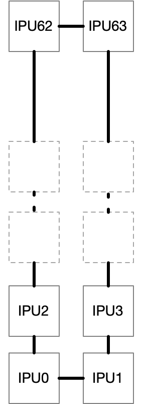
Fig. 7.6 Ring topology with replica size 1 (each IPU is a single replica)
There are a couple of ways to build a ring.
With loopback cables, we can build a direct ring (Fig. 7.7). In a direct ring, a replica communicates directly with the replicas on either side of it in the ring. In addition, the first replica (situated physically at the bottom of the Pod), communicates with the last replica (situated physically at the top of the Pod), closing the ring.
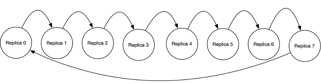
Fig. 7.7 Direct ring of replicas
At each step of the allreduce, GCL will instruct replicas to exchange data using a CrossReplicaCopy. These ring topologies are reflected in the replica map provided to that CrossReplicaCopy.
7.9.2.2. GCL allreduce with many Pods
When using many Pods, it is not possible nor efficient to form rings. Instead GCL optimises the usage of the IPU-Links and the GW-Links. The allreduce operation is split into three phases:
A reduce scatter within a Pod, after which each replica, on each Pod, has a fraction of the result for the given Pod.
An allreduce between Pods. During this phase, replicas reduce their fragment horizontally across Pods. Horizontally means with the same replica in other Pods. For example, all replica 0s, at the bottom of each Pod, allreduce their fragments together. All replica 1s, just above do the same. And so on for all replicas. After this phase, each Pod has exactly the same data.
An allgather within a Pod. This allows all replicas within a Pod to gather all the fragments within that Pod. At the end, each replica has the full reduced tensor.
During the three phase allreduce, the CrossReplicaCopies operation for the first and the third phase will have a replica map that describes IPU-Link communication. The second phase will generate CrossReplicaCopies with a replica map that describes the GW-Link communication.