5. Common algorithmic techniques for IPUs
This chapter describes some common algorithmic patterns for the IPU. Many of these patterns are used in the various ML frameworks that have been ported to the IPU (for example, TensorFlow and PyTorch). The concepts are presented here in a framework agnostic way and assume a basic knowledge of neural network training, backpropagation, and training through gradient descent. To learn more about the specific techniques that can be used with each framework, refer to the technical notes, examples and user guides for that framework available on the Graphcore documents website.
5.1. Replication
Replication is running the same program in parallel on several sets of IPUs. The program itself may be a multi-IPU program. For example, there could be a program running across four IPUs which is then replicated four times — using 16 IPUs in total (Fig. 5.1).
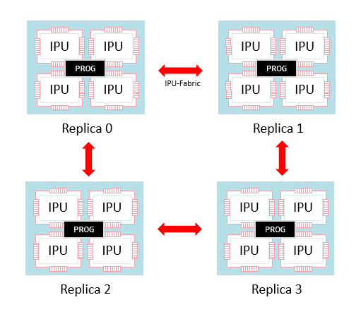
Fig. 5.1 A set of sixteen IPUs split into four replicas each running the same program
Note that the replicas are still connected by the IPU-Fabric and therefore they can communicate with each other. This communication is done via collective operations that synchronise between the replicas and swap information. An example of a collective operation is an AllReduce which, for example, takes a tensor on each replica, calculates the sum across the replicas and then creates a new tensor on each replica holding that sum.
Replicas run in a data-parallel fashion. When programs copy data to and from the host, each replica will receive and produce a different piece of data.
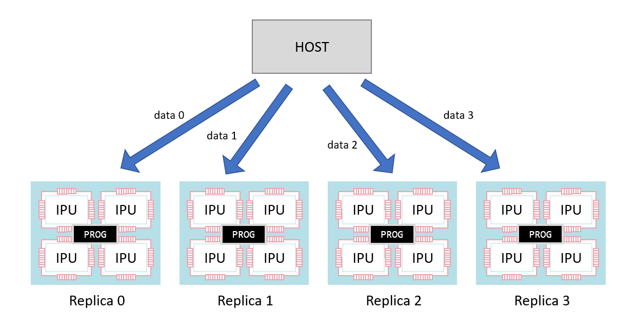
Fig. 5.2 Copies over data streams have different data for each replica
Each replica has an ID which is available to the program to direct its behaviour.
5.1.1. Replication in ML training
Replication fits naturally with data-parallel neural network optimisation. An optimisation loop will look similar to the following pseudo-code:
repeat:
  calculate forward pass of model on batch to get loss
  calculate backward pass of model to get weight gradients
  update weight using weight gradients
For data-parallel training, each replica runs the same program on different batches of data with the following modification:
repeat:
  calculate forward pass of model on batch to get loss
  calculate backward pass of model to get weight gradients
  obtain sum of gradients across all replicas
  update weight using weight gradients
Before the weight update, the sum of the gradients from each replica is calculated and distributed to all replicas (using an AllReduce operation). In some cases, the mean will be used instead of the sum.
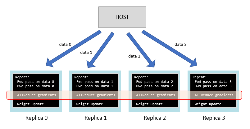
Fig. 5.3 Data parallel neural network training across replicas
The weights on each replica will start with the same value and each update will use the same aggregated gradients across the replicas. So, the weights on each replica will also hold the same values. At the end of training, the learned weights can be extracted from one of the replicas.
5.1.2. Replication in ML inference
For inference, replication is very simple — each replica runs the same inference program on different data (Fig. 5.4).
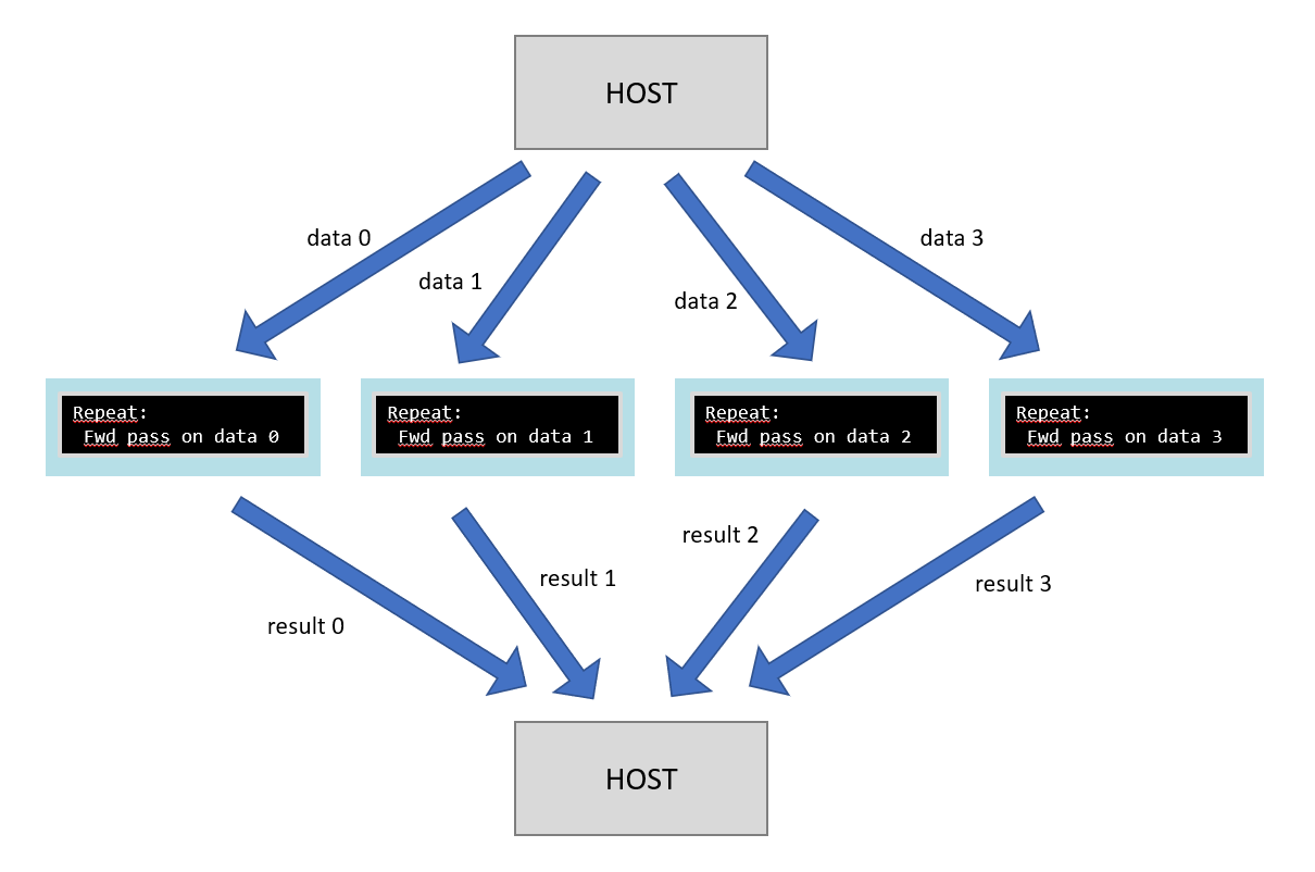
Fig. 5.4 Data parallel inference across replicas
5.1.3. Using multiple processes on the host or multiple hosts
It is possible to use multiple processes on the same host or multiple processes on different hosts connected to a set of replicas. Each process will connect to a different subset of the replicas (Fig. 5.5).
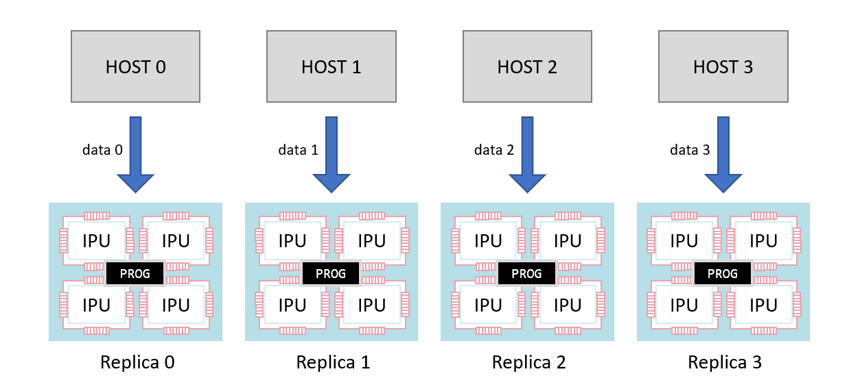
Fig. 5.5 Replicated programs with multiple hosts
This allows scaling to very large numbers of IPUs. The Poplar SDK provides a configuration library (popdist) to
configure each process to connect to its allocated replicas.
The launching of multiple processes can be performed in many ways; for example, via orchestration software such
as Kubernetes. The Poplar SDK provides a lightweight multi-host process launcher called poprun which can
also be used. For more details, refer to the PopDist and PopRun User Guide.
5.1.3.1. Replicated tensor sharding
A very general technique to reduce the memory requirement on a program is to use replicated tensor sharding. This technique works when each replica wants the same data.
In this case, the tensor containing that data can be split amongst the memories of the replicas (this may be In-Processor-Memory or Streaming Memory). Each replica will hold a section of the tensor. When the tensor needs to be used within the program, an AllGather operation will join the sections together and broadcast the full tensor to each replica (Fig. 5.6).
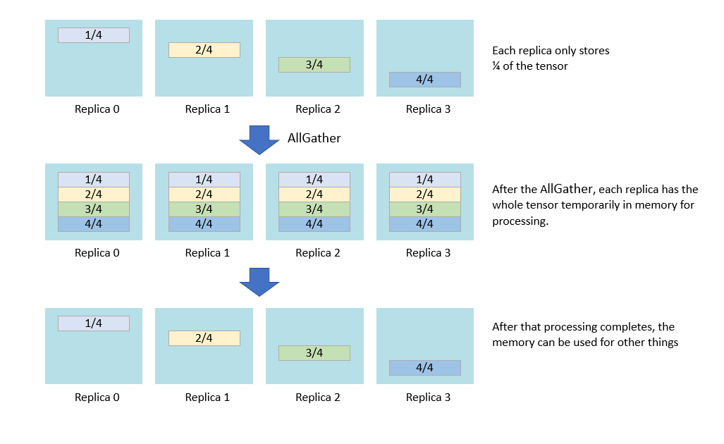
Fig. 5.6 Replicated tensor sharding
In this way, the full tensor is only in memory temporarily when it is used, not for the entire lifetime of the program. This technique trades off speed of accessing the data (since the AllGather operation needs to be performed) against overall program memory usage.
In data-parallel training, the weights and the optimiser state (for example, the exponential moving average of the gradients in the momentum optimiser) contain the same data across replicas such that you can use this technique. For example, the following pseudo-code shows how it would be used for the optimiser state.
repeat:
  calculate forward pass of model on batch to get loss
  calculate backward pass of model to get weight gradients
  obtain sum of gradients across all replicas
  perform AllGather of optimiser state across replicas
  update weights
5.2. Gradient accumulation
Gradient accumulation is a general technique for performing a step of an optimiser algorithm on a large batch consisting of many smaller batches which are executed one after the other in a loop. The gradients from processing multiple batches are accumulated and used in a single weight update step.
Recall that the pseudo-code for a training loop is:
repeat:
  calculate forward pass of model on batch to get loss
  calculate backward pass of model to get weight gradients
  update weight using weight gradients
A gradient accumulation loop would look like this:
repeat:
  zero accumulated weight gradients
  for N iterations:
    calculate forward pass of model on batch to get loss
    calculate backward pass of model to get current weight gradients
    add current weight gradients to accumulated weight gradients
  update weight using accumulated weight gradients
When not using gradient accumulation, each forward and backward pass deals with
the same size batch and therefore uses the same amount of memory. With gradient
accumulation, gradients are accumulated over multiple batches meaning that there
is a longer period between weight updates. The accumulation of gradients can be
a summation or a mean during the batch
processing loop. It is also possible to take a running mean (in some frameworks) during the batch processing loop, for example as described in the PopART (C++, Python) or PyTorch documentation.
Gradient accumulation is advantageous to amortise the cost of any replicated allreduce step in the algorithm if data-parallelism is being used.
repeat:
  zero accumulated weight gradients
  for N iterations:
    calculate forward pass of model on batch to get loss
    calculate backward pass of model to get current weight gradients
    add current weight gradients to accumulated weight gradients
  obtain sum of gradients across all replicas
  update weight using accumulated weight gradients
Gradient accumulation is also used to amortise the ramp up and ramp down phases of pipelined model parallel execution (Section 5.4.2, Efficient pipelining).
5.3. Recomputation
In neural network training, the activations calculated throughout the layers of the model need to be stored for the backward pass when gradients are calculated.
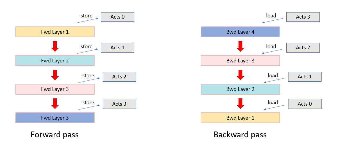
Fig. 5.7 Activation storage between the forward and backward pass
Recomputation is a general technique in which we do not store all the activations in memory. Instead it will store a subset of the activations at specified checkpoints and then recompute the intermediate activations when calculating the backward pass. This reduces the overall amount of memory required (at the cost of extra computation).
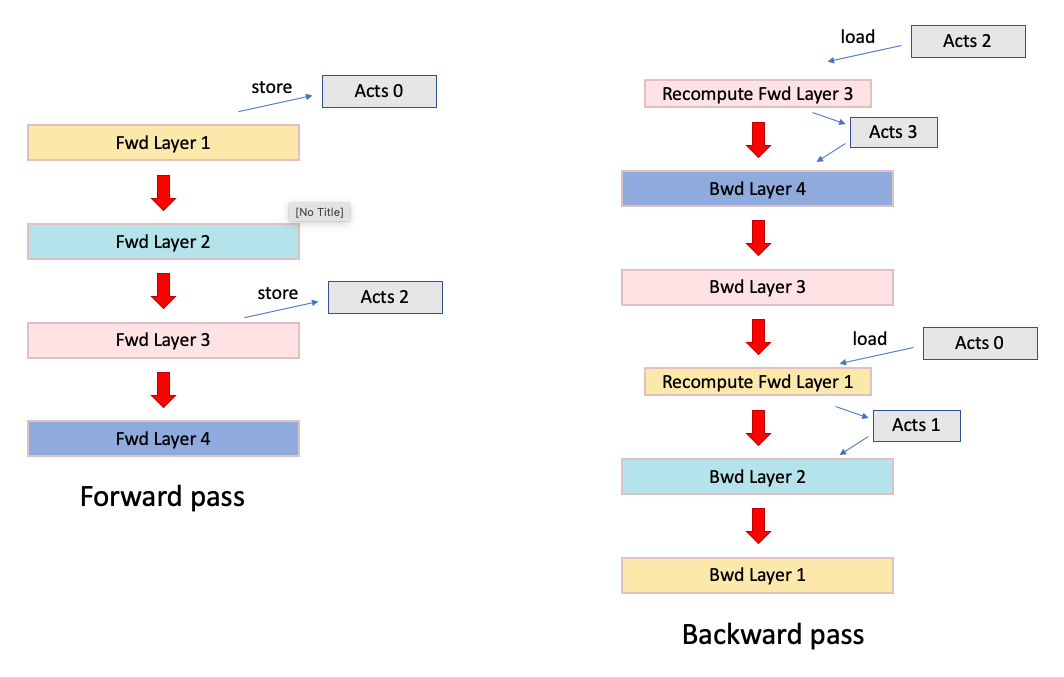
Fig. 5.8 Forward and backward pass with recomputation (in red)
Recomputation is especially effective when combined with pipelined model parallelism (Section 5.4, Model parallelism and pipelining (multi-IPU execution)).
5.4. Model parallelism and pipelining (multi-IPU execution)
On IPUs, it is common to split a model over multiple IPUs within a data-parallel replica such that each IPU executes part of the model. This is generally known as model parallelism.
Note
The number of IPUs that a model is split over must be a power of 2.
Pipelining of neural networks is a strategy to divide a model into pieces and distribute those pieces efficiently across multiple processors to be executed in parallel. There are two steps to this: split the model into independent parts consisting of sets of neural network layers and then arranging for those parts to execute in parallel.
In the case of the IPU, pipelining can enable training of large models that exceed the memory capacity on a single IPU while maintaining high IPU utilisation. Pipelining is a form of model parallelism. It can be combined with data-parallel training, implemented using replication (Section 5.1, Replication).
To implement a pipelined execution strategy, the model must be sharded across its layers. Sharding is a technique for splitting a program, and the data it processes, so that it can be run on multiple IPUs.
Since each ML framework handles pipelining in a slightly different way, this section introduces the basic concepts of pipelining in a framework-agnostic way. You can find references to information about pipelining in each framework in Section 5.4.5, Further reading on pipelining.
5.4.1. A simple example
Pipelining can be applied to both inference and training of machine learning models. Here, we will consider a simple training example.
Deep neural network training typically consists of repeated iterations of forward and backward pass computations. Each iteration processes a batch of input data to perform an update of the model parameters. The key idea of pipelining is to divide the model into pieces that process the different samples in the batch in turn; or in other words, in a pipeline. Consider a simple example that involves three IPUs, each with the weights and code of a different layer stored in its memory (Fig. 5.9).
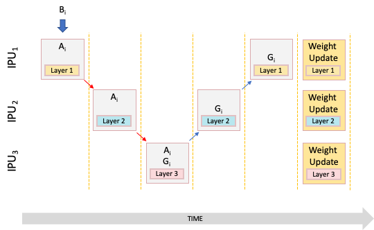
Fig. 5.9 Basic example of a pipeline
Key |
Explanation |
|---|---|
Bi |
A micro batch of data elements to be fed into the pipeline. |
Ai |
Calculation of forward activations for micro batch i. |
Gi |
Calculation of parameter gradients for micro batch i |
After IPU 1 has computed the forward activations of the first layer with respect to the first micro batch, then IPU 2 can compute the forward activations for the second layer. In other words, the batch computations are passed from pipeline stage to pipeline stage until they reach the last stage with the loss computation.
At this point, the backpropagation can commence and the IPUs can calculate the gradients of the weights for each part of the model. This executes as a pipeline in the reverse order of the forward pass. After the weight gradients are calculated, the weights can then be updated (combined with some learning rate) for the next iteration.
For gradient-descent training, a set of data items — a batch — will be processed between updates to the weights. When pipelining, we divide the batch into smaller micro batches that will be passed through the compute stages on each IPU. Each forward and backward pass will process a micro batch and the gradients will be aggregated using gradient accumulation (Section 5.2, Gradient accumulation) before doing a weight update. (Refer to Section 5.5.1, Batch size terminology for more details about the batch size terminology).
For example, if we want to train our model with a total batch size after gradient accumulation of 48, we can form 12 micro batches of size 4. The first micro batch is passed to the first IPU to compute the forward activation while all other IPUs sit idle. Fig. 5.10 shows pipelining with gradient accumulation and multiple micro batches.
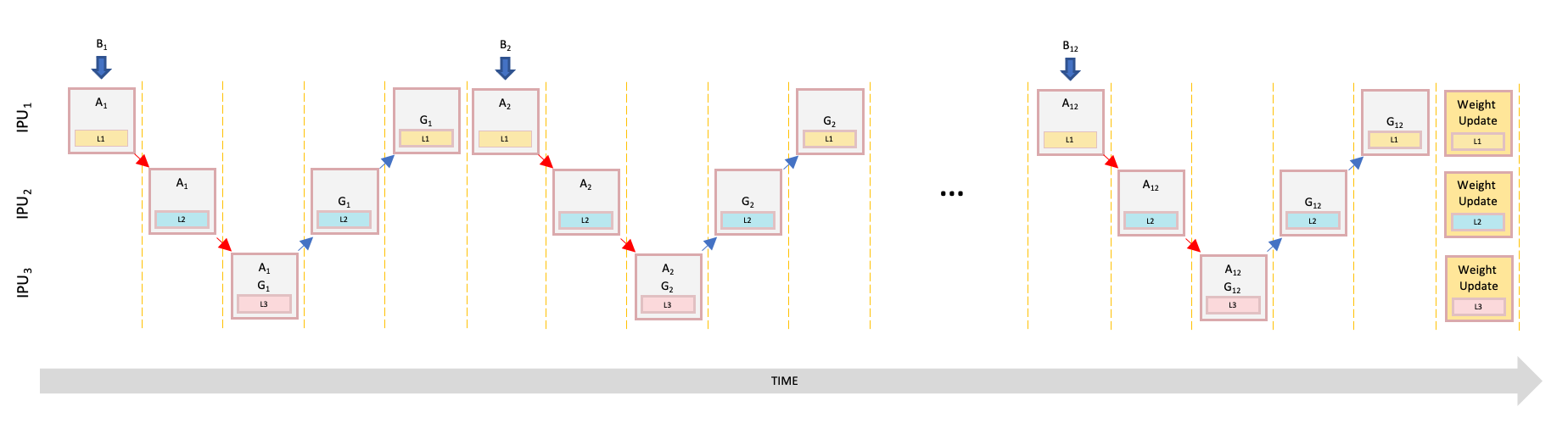
Fig. 5.10 Pipelining with gradient accumulation and multiple micro batches
5.4.2. Efficient pipelining
In the previous example, the model was simply sharded across multiple IPUs but no more than one IPU was ever used at a time whilst executing the pipeline. This has the effect of utilising memory well because the model weights are spread across the IPUs. However, the compute utilisation is not good — at any point, only one out of the three IPUs is busy. With a few modifications, we can improve this utilisation by exploiting more parallelism across the IPUs.
To get more parallelism, we can parallelise the processing of the multiple micro batches going through the pipeline when gradient accumulation is being used. For example, a batch size of 48 could be split into 12 micro batches of size 4.
After the computation of micro batch 1 in the first pipeline stage is completed, IPU 1 can start processing the next forward activation of micro batch 2. Thus, IPU 1 computes micro batch 2 in parallel to IPU 2 processing micro batch 1. Similarly, once IPU 3 starts processing micro batch 1, IPU 2 can process micro batch 2, while IPU 1 starts processing micro batch 3. At this point, the pipeline is fully ‘ramped up’ and all IPUs are computing in parallel.
As the backpropagation begins, it is important to note that we need to ensure that all micro batches are processed with respect to the same weights. With gradient accumulation the weights are not updated until all the micro batches are processed.
Once the last micro batch has been processed on IPU 3, it can apply the accumulated weight update for its layer and continue the backpropagation. After IPU 2 receives the data for the last micro batch from IPU 3, IPU 3 sits idle since there are no more incoming micro batches to process. Similarly, once IPU 2 finishes the last micro batch, it idles while IPU 1 processes the final computation in the pipeline. In other words, the pipeline ‘ramps down’ before the next iteration begins. Fig. 5.11 shows the execution of this scheme.
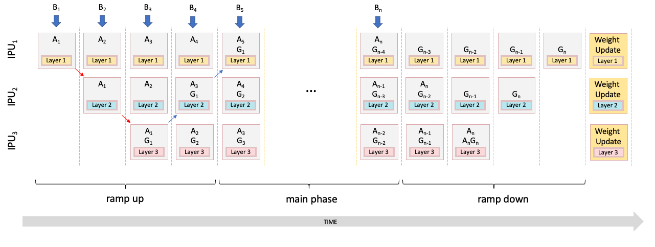
Fig. 5.11 Execution of pipelined training with IPUs running in parallel on different micro-batches
During the ramp-up and ramp-down of the pipeline, some IPUs sit idle but during the main phase of the execution (when the pipeline is fully ramped up) all IPUs are utilised. If the batch size is much larger than the number of IPUs in the pipeline, we can achieve very high IPU utilisation while minimising the ramp up and down phases. In the main phase, each IPU is running the forward pass and the backward pass of its layers at each step. To get the best utilisation, the layers across the IPUs should be balanced such that they each take roughly the same amount of time to compute.
An estimation of the level of utilisation obtained by pipelining can be quantified. For the pipeline in Fig. 5.12 with \(n\) stages, the utilisation is:
where \(T_{GA}\) is the time for a gradient accumulation, \(T_a\) is the longest time to calculate activations across all stages and \(T_g\) is the longest time to calculate gradients across all stages and \(T_{WU}\) is the time for the weight update.
In the special case when the weight update is very quick (which happens when the optimiser state is stored on the IPU) and the time for the backward pass is a fixed multiple of the time for the forward pass, then the utilisation reduces to:
If \(T_{GA} >> n\), the utilisation tends to 1.
For example, for 4 pipeline stages and only 1 gradient accumulation step then the utilisation is 1/4 = 25%. For 1000 gradient accumulation steps, then the utilisation improves to 1000/1003 = 99.7%.
The above example is only one way to schedule the execution such that the IPUs run in parallel. Section 5.4.4, Interleaved schedule pipelining shows an alternate schedule.
5.4.3. Memory stashes and recomputation
As can be seen in Fig. 5.11, on IPU 1 the weight gradients of micro batch 1 are calculated while micro batch 5 is being passed into the forward pipeline. Computing the weight gradients requires the stored activations from the forward pass. Thus, they need to be available on IPU 1 at that time. To enable this, we create a four-place queue of activations on the IPU. After the forward pass, the activations are pushed into the queue. Before the backward pass, the activations are taken from the back of the queue. This queue is called the activation stash.
The length of the stash is longest for the first IPU in the pipeline. Each subsequent IPU has its queue length reduced by 2. So, the memory requirements for the stash are largest on the first IPU. The memory required for the stash can be a significant proportion of the overall memory use.
It is possible to optimise the memory required for the stashes. By default, the stash needs to store all the intermediate activations required by the part of the model in that stage. This may be many layers — with each layer requiring a stored batch of activations. As an alternative, we can perform recomputation which can trade off computation time and memory (Section 5.3, Recomputation).
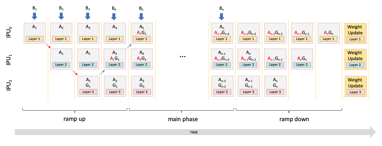
Fig. 5.12 Pipelining training with recomputation
Fig. 5.12 shows the execution of pipelining with recomputation added. When recomputation is used, the stash will only store the activations from the first layer on that IPU — greatly reducing the size of the stash. When the backward pass is needed, the forward pass is recomputed, given all the intermediate activations for that batch. This can greatly reduce the memory required at the cost of some more compute.
The recomputation of activations from the start of the layers on a particular IPU will reduce the size of the stash but memory is still needed to hold the set of recomputed activations (affecting peak live memory usage). This usage can be reduced and traded off against the size of the stash by adding extra recomputation points within the layers running on that IPU.
5.4.4. Interleaved schedule pipelining
In the previous example, on IPU 1 the weight gradients of micro batch 1 are calculated while micro batch 5 is being passed into the forward pipeline. In general, if we have \(N\) IPUs in a pipeline, the maximum stash length will be \(2\times N - 1\).
It is possible to reduce the stash lengths by scheduling the parallel computation across IPUs in a different order. Using the interleaved schedule reduces the stash length and so can be more memory efficient, but since there is an imbalance between the forward and backward stages, this may not get as good a utilisation. Therefore, this pipelining schedule is slower overall.
Fig. 5.13 shows a schedule that reduces the maximum stash to \(N\). This is known as the interleaved schedule since each step interleaves the backward pass and forward pass across the IPUs.
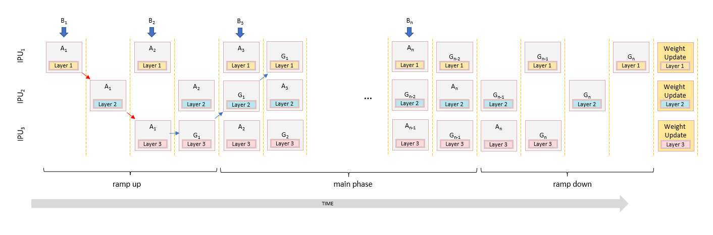
Fig. 5.13 Interleaved schedule pipelining
In this example, we can see on IPU 1 that the weight gradients of micro batch 1 are calculated while micro batch 3 is being passed onto the forward pipeline.
5.4.5. Further reading on pipelining
To learn how to use pipelining when programming the IPU using a specific framework, refer to the documentation for that framework:
PyTorch:
User Guide: Multi-IPU execution strategies
TensorFlow 2:
TensorFlow 2 API: TensorFlow 2 User Guide
TensorFlow 1:
Technical note: Model parallelism with TensorFlow: sharding and pipelining
Tutorial: TensorFlow 1 Pipelining Tutorial
Introductory example: Pipelining examples
TensorFlow 1 API:
tensorflow.python.ipu.pipelining_ops.pipeline()
PopART:
User Guide: Performance optimisation
Introductory examples: Pipelining examples
5.5. Machine learning techniques on IPU hardware
5.5.1. Batch size terminology
As noted in Section 5.4.1, A simple example, for gradient-descent training a batch of data items is processed between weight updates. When the batch is a subset of the training dataset, it may also be referred to as a mini-batch. In general, the terms batch and mini-batch are used interchangeably because it is not practical to do batch gradient descent on the entire dataset (due to the size of most datasets).
In the pseudocode above we used the terms batch and micro batch.
In our glossary we define the following terms:
Compute batch size: the number of samples for which activations/gradients are computed in parallel in a single replica. This will be smaller than the micro batch size if batch serialisation is used.
Micro batch size: the number of samples for which activations are calculated in one full forward pass of the algorithm, and for which gradients are calculated in one full backward pass (when training), in a single replica.
Replica batch size: the number of samples that contribute to a weight update from a single replica, where replica batch size = micro batch size * number of gradient accumulation iterations
Global batch size: the number of samples that contribute to a weight update across all replicas, where global batch size = replica batch size * number of replicas
If there is no gradient accumulation or replication then the micro batch size is the same as the (mini-)batch size.