16. Application example: MNIST

In this section, you will see how to train a simple machine learning application in PopXL. The neural network in this example has two linear layers. It will be trained with the the MNIST dataset. This dataset contains 60,000 training images and 10,000 testing images. Each input image is a handwritten digit with a resolution of 28x28 pixels.

16.1. Import the necessary libraries

First, you need to import all the required libraries.

import argparse
from typing import Dict, List, Tuple, Mapping
import numpy as np
import torch
from tqdm import tqdm
import popxl
import popxl.ops as ops
import popxl.transforms as transforms
from popxl.ops.call import CallSiteInfo
from mnist_utils import Timer, get_mnist_data

16.2. Prepare dataset

You can use a torch.utils.data.DataLoader for the training and validation data. Here, mnist is a function that returns a torch.utils.data.DataSet for the MNIST dataset.

    training_data = torch.utils.data.DataLoader(
        mnist(train=True),
        batch_size=batch_size,
        shuffle=True,
        drop_last=True,
    )

    validation_data = torch.utils.data.DataLoader(
        mnist(train=False),
        batch_size=test_batch_size,
        shuffle=True,
        drop_last=True,
    )

16.3. Create IR for training

The training IR is created in build_train_ir. After creating an instance of IR, operations are added to the IR within the context of its main graph. These operations are also forced to execute in the same order as they are added by using context manager :py:func:~popxl.in_sequence`.

    ir = popxl.Ir()
    ir.num_host_transfers = 1
    ir.replication_factor = 1
    with ir.main_graph, popxl.in_sequence():

The initial operation is to load input images and labels to x and labels, respectively from host-to-device streams img_stream and label_stream.

        # Host load input and labels
        img_stream = popxl.h2d_stream(
            [opts.batch_size, 28, 28], popxl.float32, name="input_stream"
        )
        x = ops.host_load(img_stream, "x")

        label_stream = popxl.h2d_stream(
            [opts.batch_size], popxl.int32, name="label_stream"
        )
        labels = ops.host_load(label_stream, "labels")

After the data is loaded from host, you can build the network, calculate the loss and gradients, and finally update the weights. This process is shown in Fig. 16.1 and will be detailed in later sections.

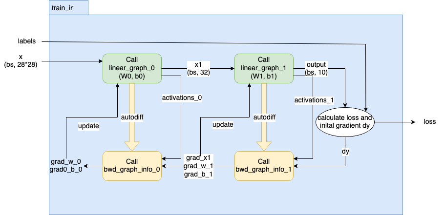
Fig. 16.1 Overview of how to build a training IR in PopXL

To monitor the training process, you can also stream the loss from the IPU devices to the host.

        # Host store to get loss
        loss_stream = popxl.d2h_stream(loss.shape, loss.dtype, name="loss_stream")
        ops.host_store(loss_stream, loss)

16.3.1. Create network

The network has 2 linear layers. A linear layer is defined by the class Linear that inherits from popxl.Module. We are here overriding the build method which builds the subgraph to do the linear computation.

class Linear(popxl.Module):
    def __init__(self) -> None:
        """
        Define a linear layer in PopXL.
        """
        self.W: popxl.Tensor = None
        self.b: popxl.Tensor = None

    def build(
        self, x: popxl.Tensor, out_features: int, bias: bool = True
    ) -> Tuple[popxl.Tensor, ...]:
        """
        Override the `build` method to build a graph.
        """
        self.W = popxl.graph_input((x.shape[-1], out_features), popxl.float32, "W")
        y = x @ self.W
        if bias:
            self.b = popxl.graph_input((out_features,), popxl.float32, "b")
            y = y + self.b

        y = ops.gelu(y)
        return y

In the diagram Fig. 16.1, you can see two graphs created from the two linear layers by using popxl.Ir.create_graph() and called by using popxl.call_with_info(). The tensors x1 and y are respectively the outputs of the first linear graph call and the second linear graph. The weight tensors, bias tensors, output tensors, graphs, and graph callsite infos are all returned for the next step. This forward graph of the network is created in the method create_network_fwd_graph.

def create_network_fwd_graph(
    ir, x
) -> Tuple[
    Tuple[popxl.Tensor], Dict[str, popxl.Tensor], List[popxl.Graph], Tuple[CallSiteInfo]
]:
    """
    Define the network architecture.

    Args:
        ir (popxl.Ir): The ir to create model in.
        x (popxl.Tensor): The input tensor of this model.

    Returns:
        Tuple[Tuple[popxl.Tensor], Dict[str, popxl.Tensor], List[popxl.Graph], Tuple[CallSiteInfo]]: The info needed to calculate the gradients later
    """
    # Linear layer 0
    x = x.reshape((-1, 28 * 28))
    W0_data = np.random.normal(0, 0.02, (x.shape[-1], 32)).astype(np.float32)
    W0 = popxl.variable(W0_data, name="W0")
    b0_data = np.random.normal(0, 0.02, (32)).astype(np.float32)
    b0 = popxl.variable(b0_data, name="b0")

    # Linear layer 1
    W1_data = np.random.normal(0, 0.02, (32, 10)).astype(np.float32)
    W1 = popxl.variable(W1_data, name="W1")
    b1_data = np.random.normal(0, 0.02, (10)).astype(np.float32)
    b1 = popxl.variable(b1_data, name="b1")

    # Create graph to call for linear layer 0
    linear_0 = Linear()
    linear_graph_0 = ir.create_graph(linear_0, x, out_features=32)

    # Call the linear layer 0 graph
    fwd_call_info_0 = ops.call_with_info(
        linear_graph_0, x, inputs_dict={linear_0.W: W0, linear_0.b: b0}
    )
    # Output of linear layer 0
    x1 = fwd_call_info_0.outputs[0]

    # Create graph to call for linear layer 1
    linear_1 = Linear()
    linear_graph_1 = ir.create_graph(linear_1, x1, out_features=10)

    # Call the linear layer 1 graph
    fwd_call_info_1 = ops.call_with_info(
        linear_graph_1, x1, inputs_dict={linear_1.W: W1, linear_1.b: b1}
    )
    # Output of linear layer 1
    y = fwd_call_info_1.outputs[0]

    outputs = (x1, y)
    params = {"W0": W0, "W1": W1, "b0": b0, "b1": b1}
    linears = [linear_0, linear_1]
    fwd_call_infos = (fwd_call_info_0, fwd_call_info_1)

    return outputs, params, linears, fwd_call_infos

16.3.2. Calculate gradients and update weights

After creating the forward pass in the training IR, we will calculate the gradients in calculate_grads and update the weights and bias in update_weights_bias.

• Calculate loss and initial gradients dy by using nll_loss_with_softmax_grad().

          # Calculate loss and initial gradients
          probs = ops.softmax(outputs[1], axis=-1)
          loss, dy = ops.nll_loss_with_softmax_grad(probs, labels)
  

• Construct the graph to calculate the gradients for each layer, bwd_graph_info_0 and bwd_graph_info_1 by using :py:func:~popxl.transforms.autodiff` (Section 10.1, Autodiff) transformation on its forward pass graph. Note that, you only need to calculate the gradients for W0 and b0 in the first layer, and gradients for all the inputs, x1, W1 and b1, in the second layer. In this example, you will see two different ways to use autodiff and how to use it to get the required gradients.

  Let’s start fromt the second layer. The bwd_graph_info_1, returned from autodiff of the second layer, contains the graph to calculate the gradient for the layer. The activations for this layer activations_1 is obtained from the corresponding forward graph call. After calling the gradient graph, bwd_graph_info_1.graph with popxl.ops.call_with_info, the grads_1_call_info is used to get all the gradients with regard to the inputs x1, W1, and b1. The method fwd_parent_ins_to_grad_parent_outs gives a mapping from the corresponding forward graph inputs, x1, W1, and b1, and their gradients, grad_x1, grad_w_1, and grad_b_1. The input gradient for grads_1_call_info is dy.

      # Obtain graph to calculate gradients from autodiff
      bwd_graph_info_1 = transforms.autodiff(fwd_call_infos[1].called_graph)
  
      # Get activations for layer 1 from forward call info
      activations_1 = bwd_graph_info_1.inputs_dict(fwd_call_infos[1])
  
      # Get the gradients dictionary by calling the gradient graphs with ops.call_with_info
      grads_1_call_info = ops.call_with_info(
          bwd_graph_info_1.graph, dy, inputs_dict=activations_1
      )
      # Find the corresponding gradient w.r.t. the input, weights and bias
      grads_1 = bwd_graph_info_1.fwd_parent_ins_to_grad_parent_outs(
          fwd_call_infos[1], grads_1_call_info
      )
      x1 = outputs[0]
      W1 = params["W1"]
      b1 = params["b1"]
      grad_x_1 = grads_1[x1]
      grad_w_1 = grads_1[W1]
      grad_b_1 = grads_1[b1]
  

  For the first layer, we can obtain the required gradients in a similar way. Here we will show you an alternative approach. We define the list of tensors that require gradients grads_required=[linears[0].W, linears[0].b] in autodiff. Their gradients are returned directly from the popxl.ops.call of the gradient graph bwd_graph_info_0.graph. The input gradient for grads_0_call_infof is the gradients w.r.t the input of the second linear graph, the output of the first linear graph, grad_x_1.

      # Use autodiff to obtain graph that calculate gradients, specify which graph inputs need gradients
      bwd_graph_info_0 = transforms.autodiff(
          fwd_call_infos[0].called_graph, grads_required=[linears[0].W, linears[0].b]
      )
      # Get activations for layer 0 from forward call info
      activations_0 = bwd_graph_info_0.inputs_dict(fwd_call_infos[0])
      # Get the required gradients by calling the gradient graphs with ops.call
      grad_w_0, grad_b_0 = ops.call(
          bwd_graph_info_0.graph, grad_x_1, inputs_dict=activations_0
      )
  

• Update the weights and bias tensors with SGD by using scaled_add_().

  def update_weights_bias(opts, grads, params) -> None:
      """
      Update weights and bias by W += - lr * grads_w, b += - lr * grads_b.
      """
      for k, v in params.items():
          ops.scaled_add_(v, grads[k], b=-opts.lr)
  
  
  

16.4. Run the IR to train the model

After an IR is built taking into account the batch size args.batch_size, we can run it repeatedly until the end of the required number of epochs. Each session is initiated by one IR as shown in the following code:

        train_session = popxl.Session(train_ir, "ipu_model")
        with train_session:
            train(train_session, training_data, opts, input_streams, loss_stream)

The session is run for nb_batches times for each epoch. Each train_session run consumes a batch of input images and labels, and produces their loss values to the host.

def train(train_session, training_data, opts, input_streams, loss_stream) -> None:
    nb_batches = len(training_data)
    for epoch in range(1, opts.epochs + 1):
        print(f"Epoch {epoch}/{opts.epochs}")
        bar = tqdm(training_data, total=nb_batches)
        for data, labels in bar:
            inputs: Mapping[popxl.HostToDeviceStream, np.ndarray] = dict(
                zip(
                    input_streams,
                    [data.squeeze().float().numpy(), labels.int().numpy()],
                )
            )

            outputs = train_session.run(inputs)
            loss = outputs[loss_stream]
            bar.set_description(f"Average loss: {np.mean(loss):.4f}")

After the training session finishes running, the trained tensor values, in a mapping from tensors to their values trained_weights_data_dict, are obtained by using train_session.get_tensors_data.

16.5. Create an IR for testing and run the IR to test the model

For testing the trained tensors, you need to create an IR for testing, test_ir, and its corresponding session, test_session to run the test. The method write_variables_data is used to copy the trained values from trained_weights_data_dict to the corresponding tensors in test IR, test_variables.

        # Build the ir for testing
        test_ir, test_input_streams, out_stream, test_variables = build_test_ir(opts)
        test_session = popxl.Session(test_ir, "ipu_model")
        # Get test variable values from trained weights
        test_weights_data_dict = get_test_var_values(
            test_variables, trained_weights_data_dict
        )
        # Copy trained weights to the test ir
        test_session.write_variables_data(test_weights_data_dict)
        with test_session:
            test(test_session, test_data, test_input_streams, out_stream)