5.2. FP8
5.2.1. IPU FP8 type
FP8, as its name implies, is an 8-bit float data type, with a memory footprint a quarter of that of FP32, half that of FP16 and the same as INT 8. The IPU supports two FP8 data types: F8E4M3 and F8E5M2.
FP8 binary encoding is shown in Table 5.1.
E4M3 |
E5M2 |
|
Exponent bias |
8 |
16 |
Max normal |
S.1111.110 = 1.75 * 2^8 |
S.11111.10 = 1.10 * 2 ^ 16 |
Min normal |
S.0001.000 = 1.0 * 2 ^ -6 |
S.00001.00 = 1.0 * 2 ^ -14 |
Max subnorm |
S.0000.111 = 0.875 * 2 ^ -6 |
S.00000.11 = 0.75 * 2 ^ -14 |
Min subnorm |
S.0000.001 = 0.125 * 2 ^ -6 |
S.00000.01 = 0.25 * 2 ^ -14 |
As can be seen from Table 5.1, the representation range of E4M3 is smaller, but the precision is slightly higher than E5M2. In addition, compared with FP32/FP16, the dynamic range of FP8 is much smaller. In order to expand the representation range, FP8 also supports adjusting the representation range using an additional scale parameter. When the scale is larger, the representation range is larger, and the precision is lower. When the scale is smaller, the representation range is smaller, and the precision is higher.
For more information about FP8, please refer to 8-bit Numerical Formats for Deep Neural Networks.
5.2.2. FP8 quantisation
Model quantisation is very common in practical applications, among which INT8 quantisation is widely applied. It is a technique that converts all inputs and parameters of the model into INT8 format with minimal loss of precision and accelerates inference speed while reducing memory footprint, mainly including post-training quantisation and quantisation training. The quantisation objects are weights and inputs, both of which introduce additional data reduction layers and increase computational complexity, unlike the direct conversion from FP32 to FP16.
The purpose of FP8 quantisation is also to minimise the loss of precision after conversion. The conversion process is as direct as that of FP32 to FP16. If the model is all FP8, there is no need to modify the model structure; simply convert the inputs and parameters to FP8. If it is a mixed precision model with FP8 and FP16, simply add Cast in the corresponding place. FP8 quantisation will determine a set of scale and format parameters to meet the requirement of minimising precision loss. At present, the IPU does not support the quantisation training of FP8, so only post-training quantisation is discussed here, including the quantisation of weights and inputs.
Regarding weight quantisation, the FP8 operators supported by IPU temporarily only include Conv, MatMul and Cast, so the weights of corresponding operators of the FP16/FP32 model will be taken out and converted into FP8. During the conversion, different scale and format parameters will be set for each set of weights. The converted weights will then be compared with the weights of FP16/FP32 to compute the loss. The corresponding scale and format of the set with the least loss are the best FP8 parameters for the weights of that layer. The subsequent set of weights will be processed in the same way. The entire conversion process is performed on the CPU, and the losses include the mean square error, mean absolute error, signal-to-noise ratio, kld and cosine distance. Simply specify one during the quantisation.
Regarding input quantisation, the quantisation principle is the same as that of weight quantisation, but the processing method is slightly different. Since the input of each FP8 operator is unknown, it is impossible to directly quantify the input. Therefore, it is necessary to provide some validation data in advance for inference, and then record the input of each FP8 operator. The next step is to find the set of scale and formats with the least loss between the input of FP16/FP32 and the input of FP8 through the traversal method, just like weight quantisation.
5.2.3. Converting an FP32 model to FP8
For operators with high computational density such as MatMul and Conv, FP8 has higher computing power than FP16. Therefore, converting the model from FP32 or FP16 to FP8 can improve model throughput and reduce model latency. In addition, since the IPU runs the entire model on the chip, and FP8 tensors require less storage space than the FP32 or FP16 tensors, the IPU can run larger scale models or support larger batch sizes.
To convert a model from FP32 or FP16 to FP8 means replacing the operator that supports FP32 or FP16 in the model with FP8 and converting the weight tensor corresponding to this operator to an FP8 tensor. Since currently in the IPU only the Conv and MatMul operators support the computation of the FP8 type, the FP8 conversion in PopRT is actually the conversion of the mixed precision model. This means, only the Conv and MatMul operators are converted to FP8, while other operators remain as the original type.
Fig. 5.1 shows an example of converting an ONNX model containing two MatMul operations to FP8. Before the MatMul operation, the output of other ops was in FP16 format, so you need to add a Cast node after these ops to convert them to FP8. Similarly, another weight input of MatMul also needed to be converted to FP8. However, the FP8 conversion of weights is not performed in the model through Cast. Instead, the FP8 conversion of weights in the ONNX model is performed on the CPU in advance, so as to save the Cast of the weight part and improve the inference efficiency. After the conversion is completed, the first FP8 MatMul is executed, and the output type is FP16. Then, when the second MatMul is executed, the input and weights will undergo the same FP8 conversion, and so on, until the entire inference process is completed.
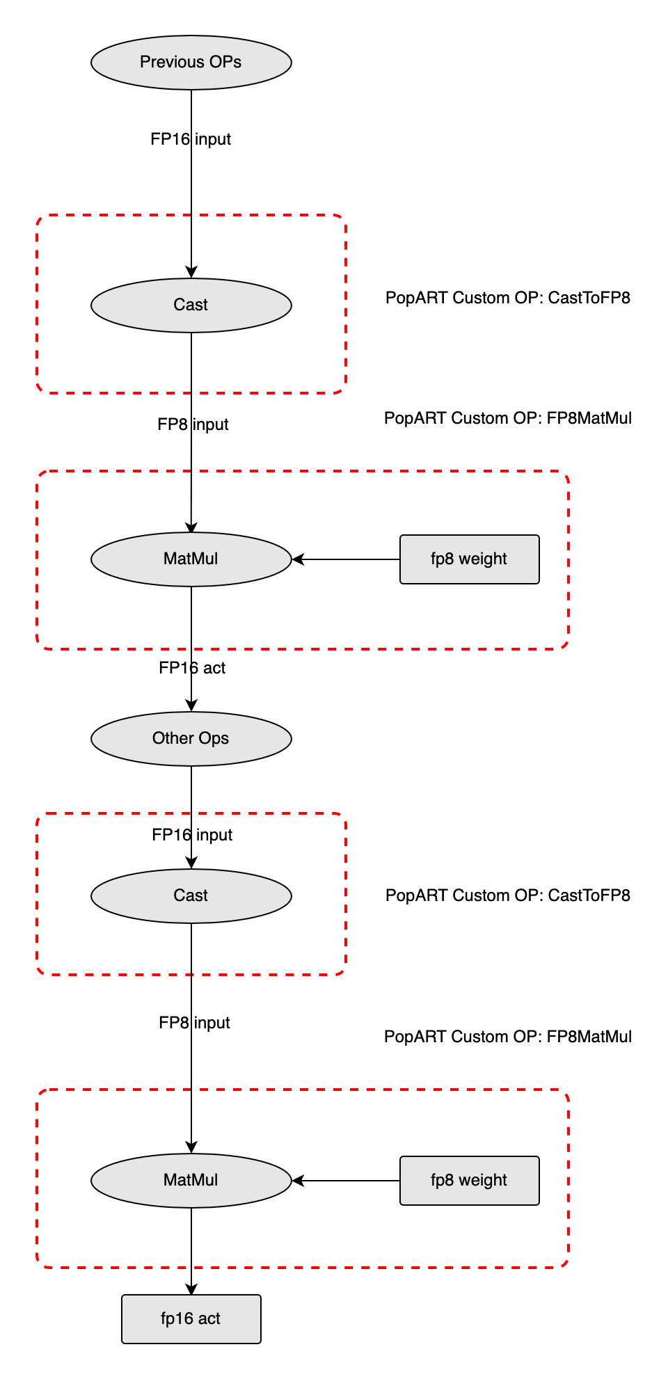
Fig. 5.1 Example showing conversion of an ONNX model to FP8
5.2.4. FP8 model conversion tool
The FP8 model conversion tool currently includes two methods of usage:
Use the default scale and format for quick conversion, with values of 0 and F143, respectively. This method can quickly verify whether the model can be successfully converted to FP8 and verify the speed of the FP8 model more conveniently.
Enable the quantisation tool of FP8 for conversion. This method will take some time to compute the best scale and format, so as to lower the precision loss of the model and to, obtain the error condition of each layer under different parameters, which facilitates further precision debugging.
We use ResNet50 as an example to demonstrate both methods.
Install the dependencies:
pip install torch==1.10.0
pip instal torchvision==0.11.1
Download the ResNet50 ONNX model and convert:
dummy_input = torch.randn((1, 3, 224, 224))
model = torchvision.models.resnet.resnet50(pretrained=True).eval()
torch.onnx.export(
    model,
    dummy_input,
    'ResNet50.onnx',
    input_names=["input"],
    output_names=["output"],
    opset_version=11,
)
The command for quick conversion is as follows:
poprt \
    --input_model ResNet50.onnx \
    --output_model ResNet50_FP8.onnx \
    --input_shape input=1,3,224,224 \
    --precision fp8 \
    --fp8_skip_op_names Conv_0,Conv_8,Gemm_121 \
    --fp8_params F143,F143,-3,-3 \
    --convert_version 11
fp8_skip_op_names and fp8_params are used to adjust precision. fp8_skip_op_names can specify which layers are retained as FP16, while fp8_params is used to specify the format and scale of inputs and weights. If these are not set, the tool will convert all Conv MatMul and Gemm operations in the model to FP8, and the format and scale will use default values.
In addition, the tool also supports using FP8 to store weights and FP16 to perform inference. Compared with the FP16 model, this method can significantly reduce memory footprint with a small increase in latency. The conversion method is basically the same as the above mentioned FP. Simply change the precision parameter to fp8_weight.
The command for quantisation conversion is:
poprt \
    --input_model ResNet50.onnx \
    --output_model ResNet50_FP8.onnx \
    --input_shape input=1,3,224,224 \
    --precision fp8 \
    --quantize \
    --quantize_loss_type kld \
    --num_of_layers_keep_fp16 3 \
    --data_preprocess calibration_dict.pickle \
    --precision_compare \
    --convert_version 11
The quantize parameter indicates that quantisation conversion is enabled, and additional input data is needed for numerical validation. num_of_layers_keep_fp16 is used to keep layers with the loss of topk as FP16 to further improve model precision.
For example, the input name of ResNet50 is input, and the input data is ImageNet. Randomly select approximately 50 images from the ImageNet test set to create a validation set, with a shape of 50*3*224*224, and then save as a pickle file in the form of a dictionary {input:ndarray}. It should be noted that if the model has preprocessing that is not included in the network, the validation data should be saved after preprocessing to ensure that it matches the input of the model.
After quantization is completed, you will get a quantize.log file which records the losses under different scales and formats of the inputs and weights of the FP8 operators. Meanwhile, the set of scales and formats with the least loss will also be given, and this set of parameters is the set of parameters used in the quantised FP8 model. In addition, when quantize_loss_type is not kld, additional information such as mean, variance, skewness or kurtosis before and after quantisation and quantisation noise will be recorded.
If precision_compare is set, the output losses of the middle layers of the FP16 model and FP8 model will be computed, and the results are saved in the precision_compare.log file, which can be used for further precision debugging. The meaning of each indicator and debugging suggestions are as follows:
Mean square error: The mean square error is used to compute the mean of the sum of squared errors between the original data and the quantised data. The closer it is to 0, the better. The value is affected by the size of the data itself and the volume of the data, so it should be considered together with the condition of the data itself.
Mean absolute error: The mean absolute error is used to compute the mean of the absolute errors between the original data and the quantised data. The closer it is to 0, the better. The value is affected by the size of the data itself and the volume of the data, so it should be considered together with the condition of the data itself.
Signal-to-noise ratio: The signal-to-noise ratio is used to compute the ratio of the sum of squared errors between the original data and the quantised data to the sum of squares of the original data. The closer it is to 0, the better. The impact of the size of the data itself and the volume of the data is eliminated, so the error condition can be judged by appropriately comparing this value for each layer.
Cosine Distance: The cosine distance is used to compute the angle between the original data and the quantised data after expansion into one dimension. The closer it is to 0, the better. It is not affected by the size of the data itself and the volume of the data, and the range is between 0 and 1. These characteristics make it a very intuitive and important evaluation indicator. This error condition can be judged by appropriately comparing this value for each layer. There may be an order of magnitude difference between some layers.
Noise skewness: Noise skewness is used to compute the skewness of the difference between the original data and the quantised data to measure the asymmetry of the distribution. If the skewness is greater than 0, the distribution is skewed to the right, and if the skewness is less than 0, the distribution is skewed to the left. Meanwhile, the larger the absolute value of skewness, the more severe the skewness of the distribution.
Noise kurtosis: Noise kurtosis is used to compute the kurtosis of the difference between the original data and the quantised data to measure the steepness or smoothness of the distribution. If the kurtosis is close to 0, the distribution kurtosis follows the normal distribution. If the kurtosis is greater than 0, the distribution is steeper, and if the kurtosis is less than 0, the distribution is shorter and fatter.
Noise histogram: The noise histogram is used to compute the difference between the original data and the quantised data. The histogram is divided into 32 bins to measure the overall distribution of the data.
Precision_compare.log provides the mean, standard deviation, minimum, maximum, skewness, kurtosis and histogram indicators of the original data, the quantised data and the error between the two. These indicators are used to characterise the overall distribution shape of the data and help users to compare the data differences before and after quantisation from a statistical perspective.
5.2.5. Debugging FP8 model conversion problems
If the precision is still poor, try the following:
For quick conversion, if it is a CV type model, it is recommended to keep the first Conv and last MatMul as FP16; if it is a NLP type model, it is recommended to keep the last MatMul as FP16. Use the F143 format as the precision of the FP8 format of E4M3 is higher in the inference process. Select an integer value between -5 and 0 for scale, and you can try to select the one with the highest precision one by one.
For quantisation conversion, the validation set should be selected from the real data, and the volume of the data should not be too large; otherwise, the quantisation process will be very long. For example, for ResNet50, approximately 20 images can be selected as the validation set. The actual situation needs to be adjusted according to the size of the model; if the quantisation speed is too slow, the volume of the data can be appropriately reduced.