Note: Searching from the top-level index page will search all documents. Searching from a specific document will search only that document.
Find an exact phrase: Wrap your search phrase in "" (double quotes) to only get results where the phrase is exactly matched. For example "PyTorch for the IPU" or "replicated tensor sharding"
Prefix query: Add an * (asterisk) at the end of any word to indicate a prefix query. This will return results containing all words with the specific prefix. For example tensor*
Fuzzy search: Use ~N (tilde followed by a number) at the end of any word for a fuzzy search. This will return results that are similar to the search word. N specifies the “edit distance” (fuzziness) of the match. For example Polibs~1
Words close to each other:~N (tilde followed by a number) after a phrase (in quotes) returns results where the words are close to each other. N is the maximum number of positions allowed between matching words. For example "ipu version"~2
Logical operators. You can use the following logical operators in a search:
+ signifies AND operation
| signifies OR operation
- negates a single word or phrase (returns results without that word or phrase)
PopRT supports sharding the ONNX graph across different devices based on provided sharding nodes to achieve model parallelism. It is suitable for large models that exceed the memory limits of a single device and require multiple devices to run.
Auto-sharding selects the alternative sharding nodes from the ONNX graph. The selection strategy selects a node in the ONNX graph that has multiple intermediate inputs, which does not include model inputs and constant inputs.
The list of alternative nodes satisfies topological sorting, and the subgraph corresponding to the alternative node is found by traversing the path from each alternative node to its input direction.
Each alternative node corresponds to a subgraph, and each subgraph records the corresponding memory (bytes_cost) and computation (FLOPs_cost):
memory (bytes_cost): sum of initialiser input sizes for all nodes in the subgraph.
computation (FLOPs_cost): sum of FLOPs of all nodes in the subgraph. The corresponding FLOPs of each node is obtained through poprt.profile.Profiler.get_profiler().
Merge the alternative nodes that have less memory or computation, so as to reduce the number of alternative nodes and improve the traversal efficiency of the sharding scheme.
Note
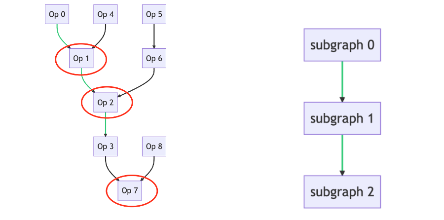
The traversal strategy of the sharding scheme is to traverse the subgraph corresponding to the alternative node as the minimum unit. The list of subgraphs still satisfies the topological sorting.
As shown in the following figure, the alternative nodes are Op1, Op2, Op7. The subgraph corresponding to Op1 is [Op1, Op0, Op4], the subgraph corresponding to Op2 is [Op2, Op5, Op6], and the subgraph corresponding to Op7 is [Op7, Op3, Op8]. Traverse from the left image to the right image.
Auto-sharding will select the sharding scheme from the alternative nodes:
Initial sharding: The list of subgraphs satisfies the topological sorting. The list of subgraphs is directly divided by subgraph memory (bytes_cost) to ensure memory balance. As shown below, divide the list of subgraphs into four subgraph groups, with each subgraph group corresponding to one IPU.
If Out Of Memory (OOM) occurs, adjust the subgraph group corresponding to the IPU that went OOM according to the memory, and try to put the removable subgraphs in this subgraph group into the adjacent or parallel subgraph group respectively for compilation.
If the sharding scheme with better performance is selected, balance the subgraph group according to the computation, try to put the removable subgraphs in the subgraph group with the largest computation into the adjacent or parallel subgraph group respectively, and search for a more computationally balanced sharding scheme for compilation.
The update of the subgraph group has the following situations:
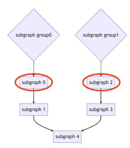
The starting subgraph of each subgraph group can be moved into the corresponding parent subgraph group. As shown below, subgraph 0 can be moved into the parent subgraph group, subgraph group 0, and subgraph 2 can be moved into parent subgraph group, subgraph group 1.
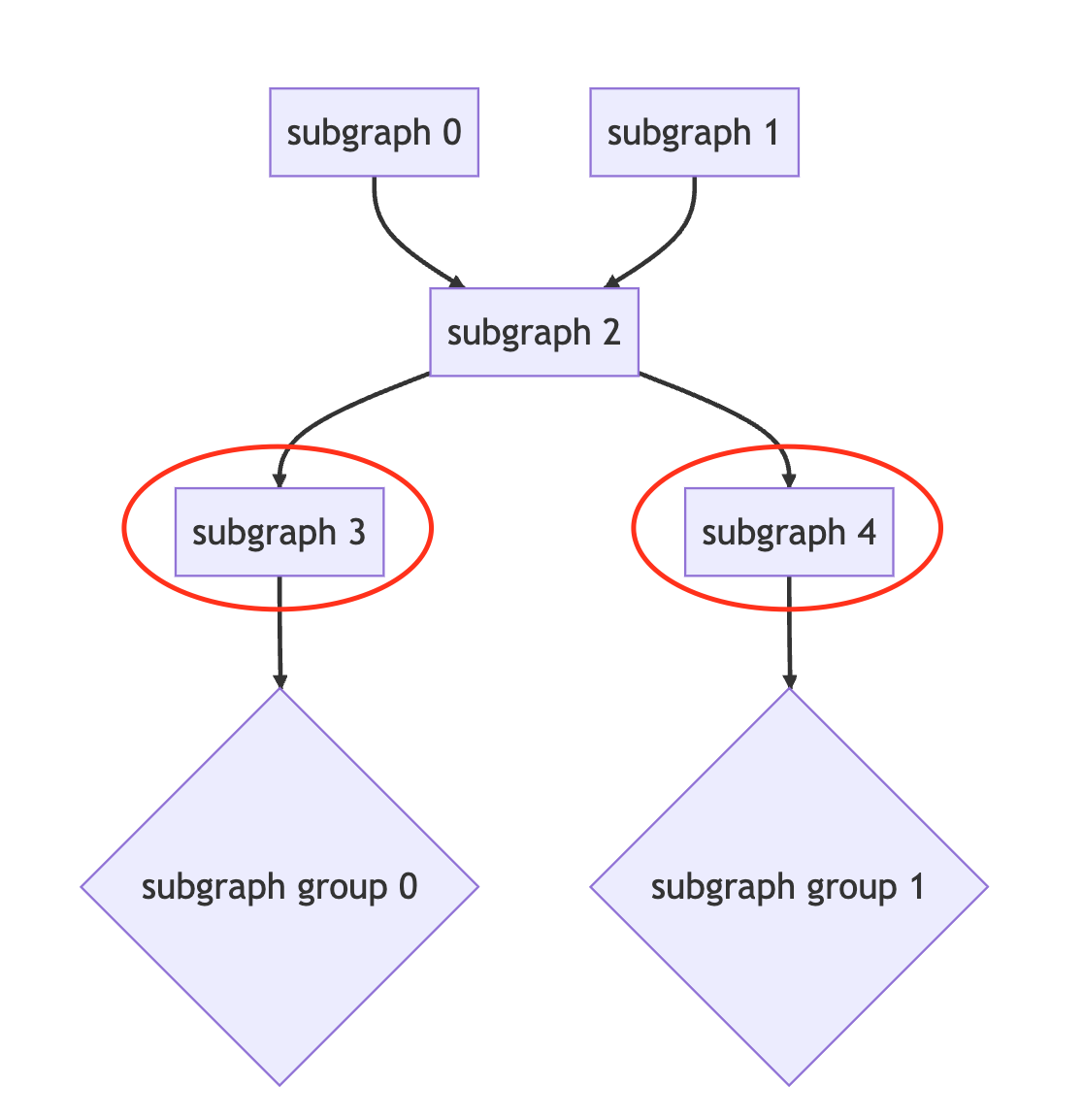
The ending subgraph of each subgraph group can be moved into the corresponding child subgraph group . As shown below, subgraph 3 can be moved into child subgraph group, subgraph group 0, and subgraph 4 can be moved into child subgraph group, subgraph group 1.
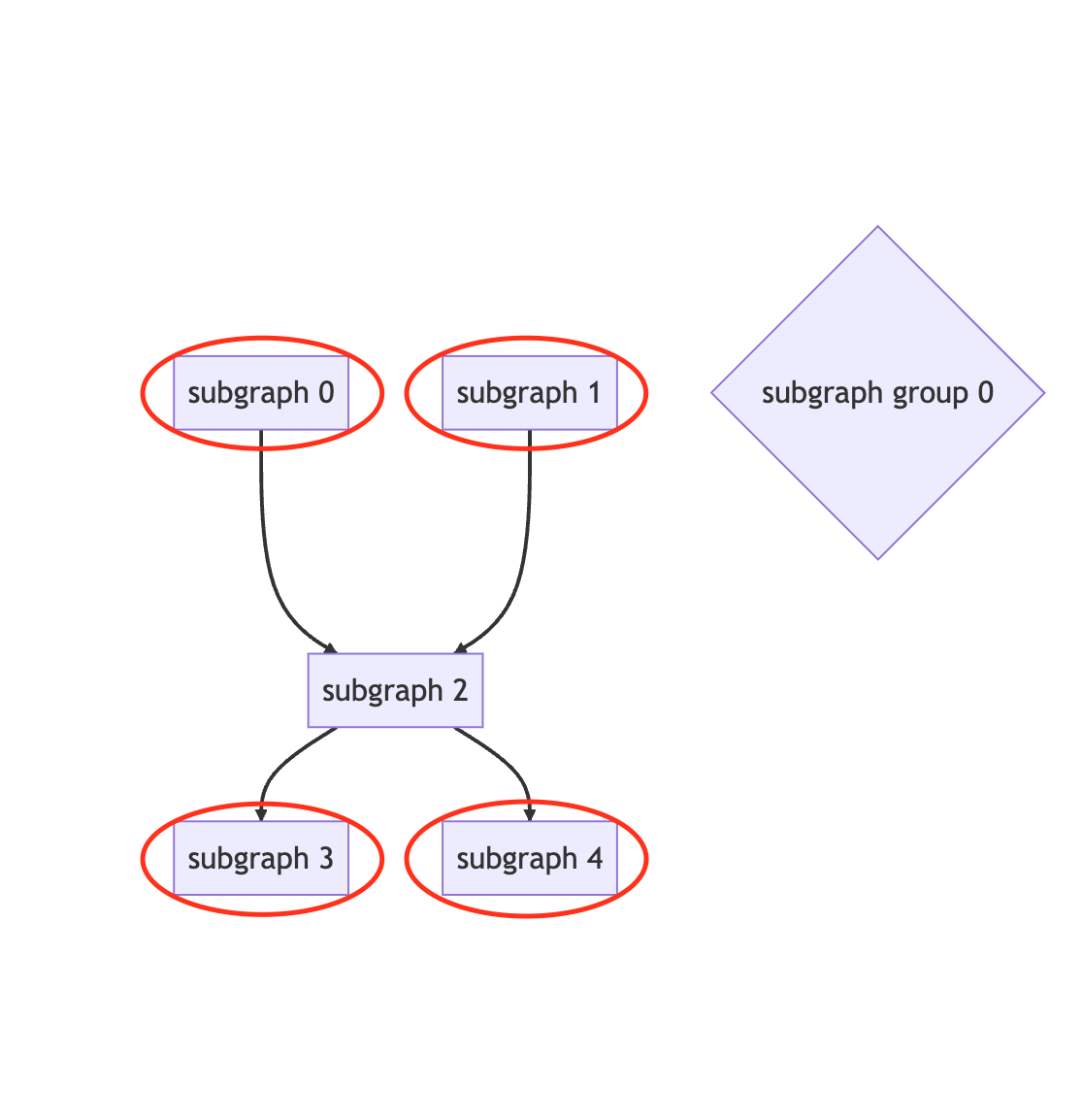
The starting subgraph or ending subgraph of each subgraph group can be moved into the corresponding parallel subgraph group. As shown below, subgraphs 0, 1, 3 and 4 can be moved into parallel subgraph group subgraph group 0.
Adjustment of available memory promotion: If an OOM occurs in each sharding scheme in the traversal strategy, select the sharding scheme with the smallest OOM size, and try to reduce the available memory proportion to 0.3 and 0.1 for compilation.
Auto-sharding requires that the input ONNX model be converted in PopRT (Quick start).
Regarding the compilation options, if the input ONNX model is FP16, partials_type defaults to half. available_memory_proportion performs the sharding strategy traversal based on the default values. If all the sharding strategies in the traversal are OOM, adjust the value for available_memory_proportion according to the aforementioned method and re-try the compilation. Apart from that, do not consider other compilation options. You can manually adjust compilation options based on the auto-sharding sharding scheme.
Since the actual performance of the sharding scheme Profiling is not considered for adjustment, the sharding scheme found by auto-sharding attempting to traverse the compilation strategy may be a locally effective solution, but not necessarily a globally optimal solution. You can use Manual Sharding to manually adjust the sharding nodes based on the sharding scheme selected by auto-sharding.
The time taken for auto-sharding is proportional to the graph compilation time. This time can be very long.
You can download the auto-sharding tool from GitHub: auto_sharding.py .
The parameters are:
--input_model${INPUT_MODEL}: The input ONNX model.
--num_ipus${NUM_IPUS}: Specify the number of IPUs
--output_model${OUTPUT_MODEL}: The output ONNX model. If not set, this will default to ${input_model}.auto_sharded.onnx.
--optimal_perf: Indicates whether to enable performance optimisation. If not enabled, the traversal will stop after finding the first successfully compiled sharding scheme. If enabled, the best performing sharding scheme will be selected after traversing all sharding schemes.
--num_processes${NUM_PROCESSES}: The number of processes for parallel compilation. Default: 2.
Performance optimisation is not enabled. Shard the model across two IPUs. All the traversal sharding schemes are OOM. Select the sharding scheme with the smallest OOM size, try available_memory_proportion=0.3, and the compilation is successful.
python auto_sharding.py --input_model ../debug/deberta.onnx.optimized.onnx --num_ipus 2...[Success] Compile successfully available_memory_proportion 0.3 and solution:Sharding nodes: Device 0 - ['Add_938'][Success] The latency 336.2899446487427 ms, tput 2.9736244449548064[Success] Save the sharded model to ../debug/deberta.onnx.optimized.onnx.auto_sharded.onnx
Performance optimisation is enabled. Shard the model across two IPUs, and the optimal solution is returned after traversal.
python auto_sharding.py --input_model=vit_l_16_16.onnx.optimized.onnx --num_ipus=2 --optimal_perf...[Success] The optimal solution:Sharding nodes: Device 0 - ['/encoder/layers/encoder_layer_11/Add_1'][Success] The optimal latency 2.712721824645996 ms, tput 368.6334481164495[Success] Save the sharded model to vit_l_16_16.onnx.optimized.onnx.auto_sharded.onnx