5.4. Poplar Tutorial 4: Profiling Output

In this tutorial you will:

learn about the different methods with which we can extract profiling information from a Poplar program;
learn and test each method with a given simple example program;
see how changes to the given program reflect into the profiles;
dive into how to use and understand the different sections of the PopVision Graph Analyser.

A brief summary and a list of additional resources are included at the end this tutorial.

Setup

In order to run this tutorial on the IPU you will need to have a Poplar SDK environment enabled (see the Getting Started Guide for your IPU system).

You will also need a C++ toolchain compatible with the C++11 standard, build commands in this tutorial use GCC.

Profiling on the IPU

There are three ways of profiling code for the IPU:

outputting summary profile data to the console.
using the PopVision Analysis API to query profile information in C++ or Python (coverage in this tutorial is a preview).
using the PopVision Graph Analyser tool.

The PopVision Graph Analyser provides much more detailed information, as such this tutorial is split into 3 parts. First we try the three different profiling methods, next we show general PopVision Graph Analyser functionality, and finally we explore each tab of information in the PopVision Graph Analyser.

The profiling tool is documented in the PopVision Graph Analyser User Guide. This tutorial shows how to profile Poplar programs, but these techniques are applicable to the PyTorch and TensorFlow frameworks.

Download and install the PopVision Graph Analyser from the developer page. You can download and install the PopVision Graph Analyser on your local machine and use it to access files on remote machines, so you do not need to download and install the PopVision Graph Analyser on your remote machines.

It is also useful to watch the Getting Started with PopVision video both before the tutorial as a preview, and after to give you further things to try.

Running on IPUModel vs IPU hardware: As with earlier tutorials, this tutorial uses the IPUModel as the default to allow you to run the tutorial even without access to IPU hardware. There are some differences between the IPUModel and IPU hardware, which will be discussed at the point they become relevant.

Tutorial 1 provides an explanation of how to modify the tutorial code to run on IPU hardware, but for this tutorial we provide code examples for both - tut4_ipu_model.cpp and tut4_ipu_hardware.cpp. We’ll reference tut4_ipu_model.cpp, but unless noted, the instructions are the the same for tut4_ipu_hardware.cpp (except the filename).

Use tut4_profiling as your working directory. This tutorial is not about completing code; the aim is to understand and experiment with the profiling options presented here.

Profiling methods

Command line profile summary

Open your copy of the file tut4_profiling/tut4_ipu_model.cpp in an editor.

Note the printProfileSummary line in the tutorial code:
```
engine.printProfileSummary(std::cout, {{"showExecutionSteps", "true"}});
```
This outputs the command line Profile Summary. Enabling the showExecutionSteps option means our profile summary will also contain the program execution sequence with cycle estimates for IPUModel, or measured cycles for IPU hardware. However, on hardware we must enable instrumentation otherwise cycles will not be recorded. Look for the debug.instrument engine option in tut4_ipu_hardware.cpp to see how instrumentation is enabled.
Compile and run the program. Note that you will need the PopLibs libraries poputil and poplin in the command line:
```
$ g++ --std=c++11 tut4_ipu_model.cpp -lpoplar -lpopops -lpoplin -lpoputil -o tut4
$ ./tut4
```
The code already contains the addCodelets functions to add the device-side library code. See the PopLibs section of the Poplar and PopLibs User Guide for more information.

When the program runs it prints profiling data. You can redirect this to a file to make it easier to study.

Take some time to review and understand the execution profile. For example:

Determine what percentage of the memory of the IPU is being used
Determine the number of cycles the computation took
Determine which steps belong to which matrix-multiply operation
Identify how many cycles are taken by communication during the exchange phases

See the Profile Summary section of the Poplar and PopLibs User Guide for further details of the profile summary.

Generating profile report files

Create a report:

(Optional) First comment out the printProfileSummary line in the tutorial code:
```
engine.printProfileSummary(std::cout, {{"showExecutionSteps", "true"}});
```
This is not needed when using the PopVision Graph Analyser, but doesn’t conflict with it either. Generating profile report files is enabled by poplar engine options, which can be changed using the api or environment variables.

Recompile:

$ g++ --std=c++11 tut4_ipu_model.cpp -lpoplar -lpopops -lpoplin -lpoputil -o tut4

Run with the following command, setting these environment variables:
```
$ POPLAR_ENGINE_OPTIONS='{"autoReport.all":"true","autoReport.directory":"./report"}' ./tut4
```
- autoReport.all turns on all the default profiling options.
- autoReport.directory sets the output directory, relative to the current directory.
You should see a new directory report in your current directory. It will contain some files (profile.pop and debug.cbor). Which files are created depends on which profiling options you have turned on.

Making use of these files is explained in the following sections. They can be used with either the PopVision Analysis API or explored with the PopVision Graph Analyser Tool.

Using the PopVision analysis API in C++ or Python

This section explains how the PopVision analysis API (libpva) can be used to query information from a profile file using C++ or Python. You can find more information in the PopVision Analysis Library (libpva) User Guide.

libpva is used to query profile.pop files, so copy your profile.pop file created in the previous section to the tut4_profiling/libpva directory and make this your working directory.

You should now see three files in your current working directory:

cpp_example.cpp - Example C++ program that queries a profile.
profile.pop - Example profile file.
python_example.py - Example Python program that queries a profile.

Study the C++ and Python source files to understand how they work. Compile the C++ program with:

$ g++ --std=c++11 cpp_example.cpp -lpva -ldl -o cpp_example

Now you can run the C++ program with:

$ ./cpp_example

Or you can run the Python program with:

$ python3 python_example.py

Both programs should print the same example information similar to this:

Example information from profile: Number of compute sets: 9 Number of
tiles on target: 1472 Version of Poplar used: 2.3.0 (d9e4130346)

You may want to modify the source files to extend this example information.

Using PopVision Graph Analyser - loading and viewing a report

Open the PopVision Graph Analyser application that you’ve downloaded from the developer page.

Load the profile in the PopVision Graph Analyser.
- You can either open a local copy of the report folder above, or open it remotely via ssh.
- Launch the PopVision Graph Analyser, and click on 'Open a Report..'.
- Navigate to either the local or remote copy of the folder.
- Click Open - this opens into the Summary tab, you can also open a specific file and it will take you straight to the corresponding tab.
You should see the Summary tab: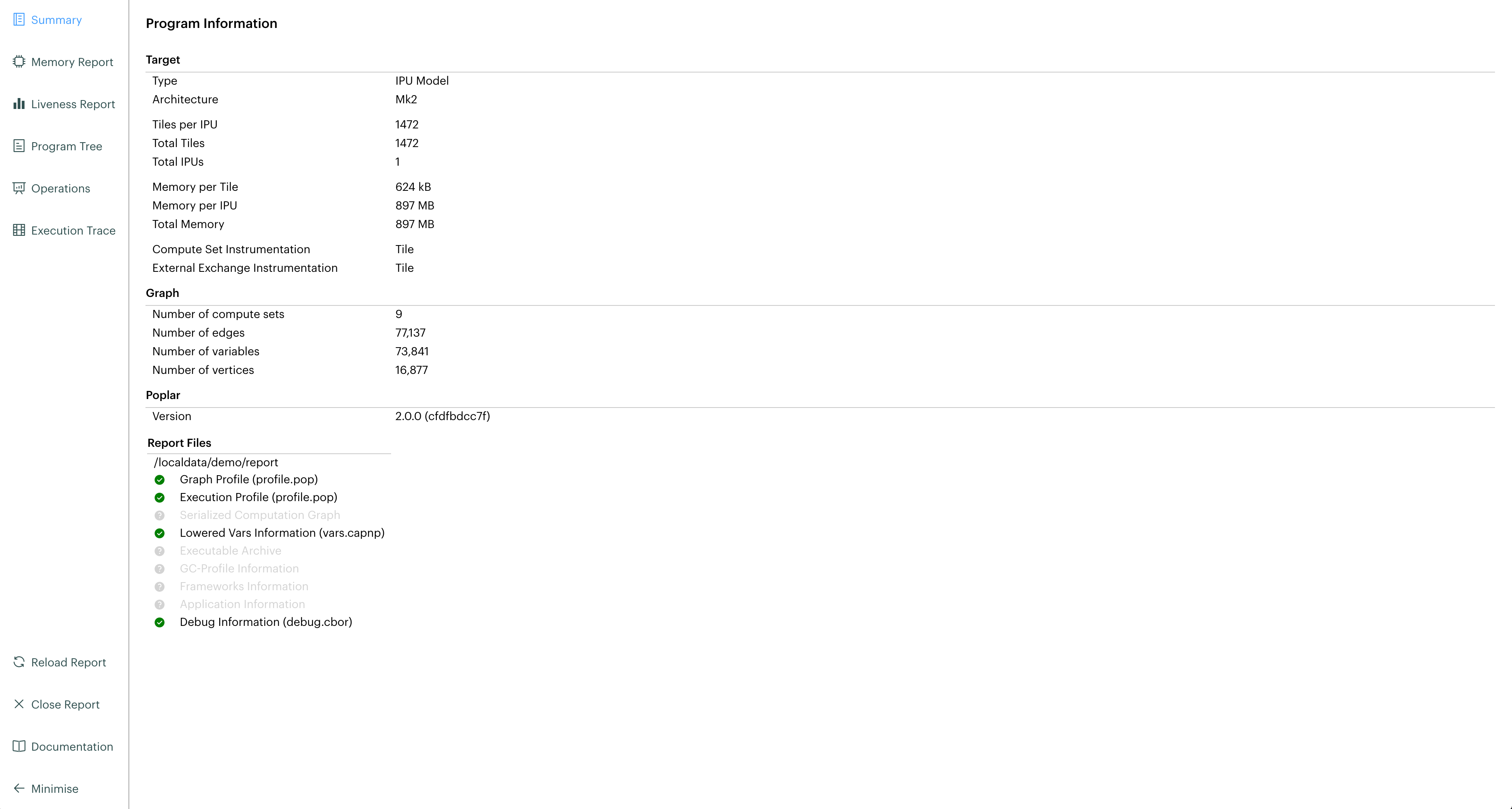
There are multiple tabs that can be opened via the icons on the left hand side of the trace - Summary, Memory Report, Liveness Report, Program Tree, Operations Summary, Operations Graph, Computations Graph and Execution Trace. The Execution Trace tab for example should look like: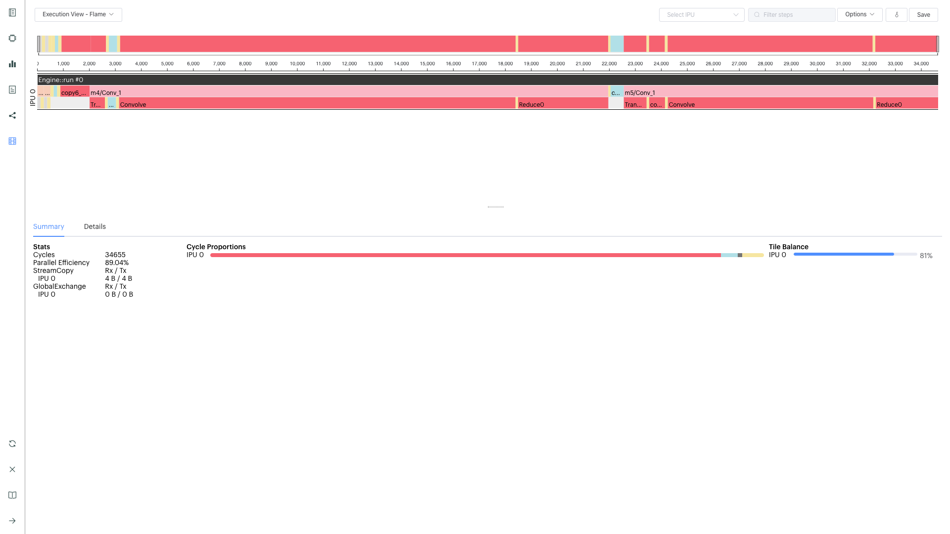
Click through the different tabs and mouse around to investigate some of the functionality. Hovering over most things gives a tool tip or a link to the documentation. This documentation is contained both in the the application itself (Help -> Documentation or the documentation icon, bottom left) and in the PopVision Graph Analyser User Guide.
The whole report can be reloaded by:
- the reload icon (bottom left).
- closing the report and re-opening it (close icon, bottom left).
- directly opening a new file (File -> Open New Window).

Using PopVision Graph Analyser - general functionality

This section of the tutorial is an introduction to the basic functionality -the PopVision Graph Analyser User Guide gives full detailed instructions.

Capturing IPU Reports - setting `POPLAR_ENGINE_OPTIONS`

The amount and type of profiling data captured is set with the POPLAR_ENGINE_OPTIONS environment variable. The default POPLAR_ENGINE_OPTIONS='{"autoReport.all":"true"}' captures all the default profiling information apart from the serialized graph.

If you only want to collect specific aspects of the profiling data, you can turn each one on individually:

$ POPLAR_ENGINE_OPTIONS='{"autoReport.outputGraphProfile":"true"}'

Conversely, if you want to exclude specific aspects, you can set autoReport.all to true, and individually disable them:

$ POPLAR_ENGINE_OPTIONS='{"autoReport.all":"true", "autoReport.outputExecutionProfile":"false"}'

The environment variables can be made to persist using export, however common use is to specify them on the same line as the program to be profiled to scope them. Experiment with turning different profiling functionality on and off. Note that the Poplar program only overwrites those files in the folder that correspond to the functionality turned on for that run. So it won’t delete files that aren’t written in that run.

This is fully detailed in the Capturing IPU Reports section of the PopVision Graph Analyser documentation.

Comparing two reports

Another useful function is the ability to compare two reports directly. Instead of clicking 'Open a Report…' in the main menu, simply click on 'Compare two Reports…', navigate the file open windows to the two reports and click Compare. For this you’ll need two reports, so modify the dimensions of one or more of the tensors, for example m1 {900, 600} -> {1600, 700}, m2 {600, 300} -> {700, 300}.

Recompile and capture a second report to a second directory:

$ g++ --std=c++11 tut4_ipu_model.cpp -lpoplar -lpopops -lpoplin -lpoputil -o tut4
$ POPLAR_ENGINE_OPTIONS='{"autoReport.all":"true","autoReport.directory":"./report_2"}' ./tut4

Compare the original report you created and your 2nd report. Look at the Summary, Memory and Liveness tabs to start with. The Liveness tab for example should look like:

We will use this extra report in the next couple of sections as well.

If you face any difficulties, a full walkthrough of opening reports is given in the Opening Reports section of the PopVision Graph Analyser documentation.

Profiling an out of memory program

If you are using hardware, and your program doesn’t fit on the IPU tiles, you will hit an Out Of Memory (OOM) error. This occurs during the graph-compilation step of running your program (not during the g++ compilation, but when actually running your program).

The IPUModel is designed not to stop for OOM errors (it can be used for building and running models that are OOM), so for this section we’ll assume you’re using hardware.

If we make tensor m1 a lot bigger (and adjust m2 to match), we can induce OOM:
```
Tensor m1 = graph.addVariable(FLOAT, {9000, 7500}, "m1");
Tensor m2 = graph.addVariable(FLOAT, {7500, 300}, "m2");
```
(remember this is on hardware, so modify tut4_ipu_hardware.cpp).

Recompile, and then run with a new folder for the report:

$ g++ --std=c++11 tut4_ipu_hardware.cpp -lpoplar -lpopops -lpoplin -lpoputil -o tut4
$ POPLAR_ENGINE_OPTIONS='{"autoReport.all":"true","autoReport.directory":"./report_OOM"}' ./tut4

You will see the program fail with an out of memory error:

terminate called after throwing an instance of 'poplar::graph_memory_allocation_error'
what():  Out of memory: Cannot fit all variable data onto one or more tiles. Profile saved to: ./report_OOM/profile.pop

And the folder /report_OOM contains a set of profile files.

Note: As of the 2.1 release of the Poplar SDK, the value of the Poplar engine option “debug.allowOutOfMemory” is set to true by default. This allows the compilation to finish when OOM is encountered, generating the profile file containing the memory trace that can be analysed. It is important to note that although a usable set of profiling files is generated, the compilation won’t succeed and execution won’t happen. This means that even if you use “autoReport.all”:”true”, you won’t get an execution trace. If the “debug.allowOutOfMemory” option is set to false, then when the program execution fails with an OOM error, the compilation will be halted, and no profile file will be created that can be analysed.

When you open the report in /report_OOM with the PopVision Graph Analyser you will see that the memory trace is complete. We could now investigate what has caused the program to go OOM and potentially fix it.

Using PopVision Graph Analyser - different tabs in the application

The next part of the tutorial takes a deeper look at each tab and the information they contain.

Memory report

The Memory Report tab allows you to investigate memory utilisation across the tiles. Open one of your reports from above, and click on the Memory Report tab icon on the left.

You should see the Memory Report tab: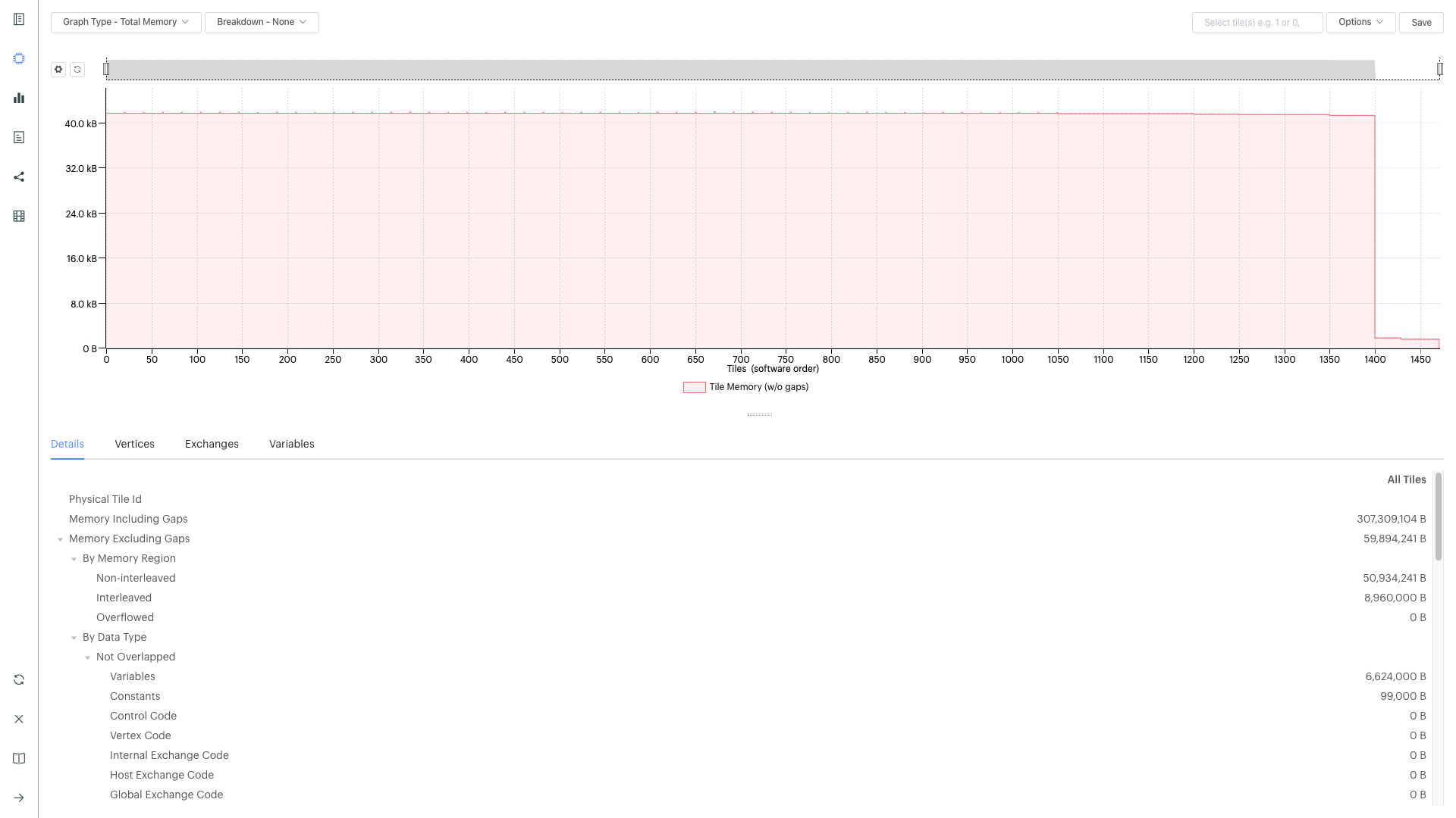

See how the Details section shows data for all tiles.
With your mouse hovering over the graph, scroll with the mouse wheel up and down and see how this zooms in and out on regions of tiles.
In the top right there is a Select tile box - type in a tile you are interested in and see how the Details section shows details on just that specific tile.
- You can enter multiple tile numbers, comma separated, to compare two or more different tiles.
- You can also Shift-click on the lines of the graph to achieve the same behaviour.
In the top right there is also a set of options. Turn on Include Gaps and Show Max Memory.
- Show Max Memory shows the maximum available memory per tile - if one or more tiles are over, it goes OOM.
- Include Gaps shows the gaps in memory - some memory banks in IPU tiles are reserved for certain types of data. This leads to ‘gaps’ appearing in the tile memory.
- The gaps can be enough to push you OOM, so it is useful to have both of these on when investigating an OOM issue.
Compare your two reports, with Show Max Memory and Include Gaps turned on.
Vary the tensors and the mapping - you can see the effects in the Memory tab of the tool.

Full details of the Memory Report are given in the Memory Report section of the PopVision Graph Analyser documentation.

Program tree

The Program Tree tab allows you to visualise your compiled code. It shows a hierarchical view of the steps in the program that is run on the IPU. Open one of your reports from above, and click on the Program Tree tab icon on the left.

You should see the Program Tree tab: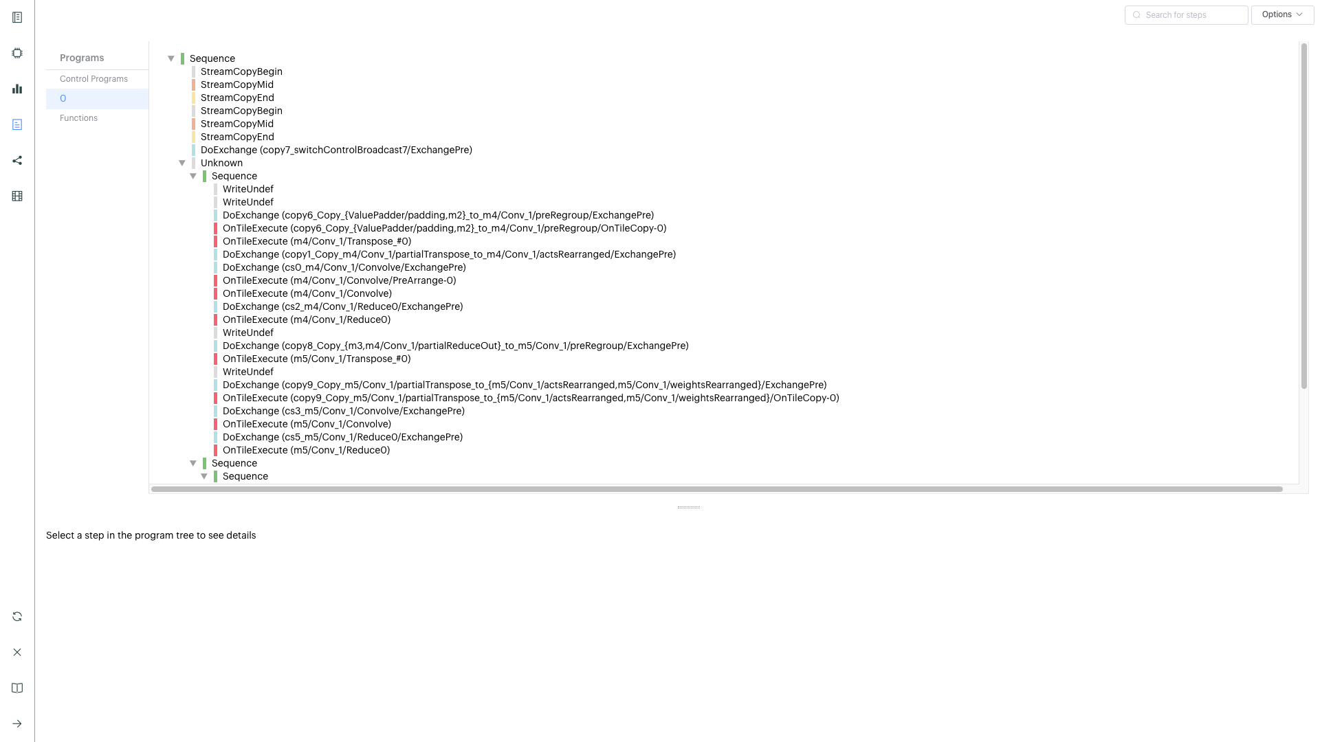
Observe the sequences of stream copies, exchanges and on-tile-executions.
Clicking on each line in the top panel gives full details in the bottom panel -observe the different info given for each type.

More details on the Program Tree are given in the Program Tree section of the PopVision Graph Analyser documentation.

Operations summary

The Operations Summary tab displays a table of all operations in your model, for a software layer, showing statistics about code size, cycle counts, FLOPs and memory use. Open one of your reports from above, and click on the Operations tab icon on the left.

You should see the Operations Summary tab: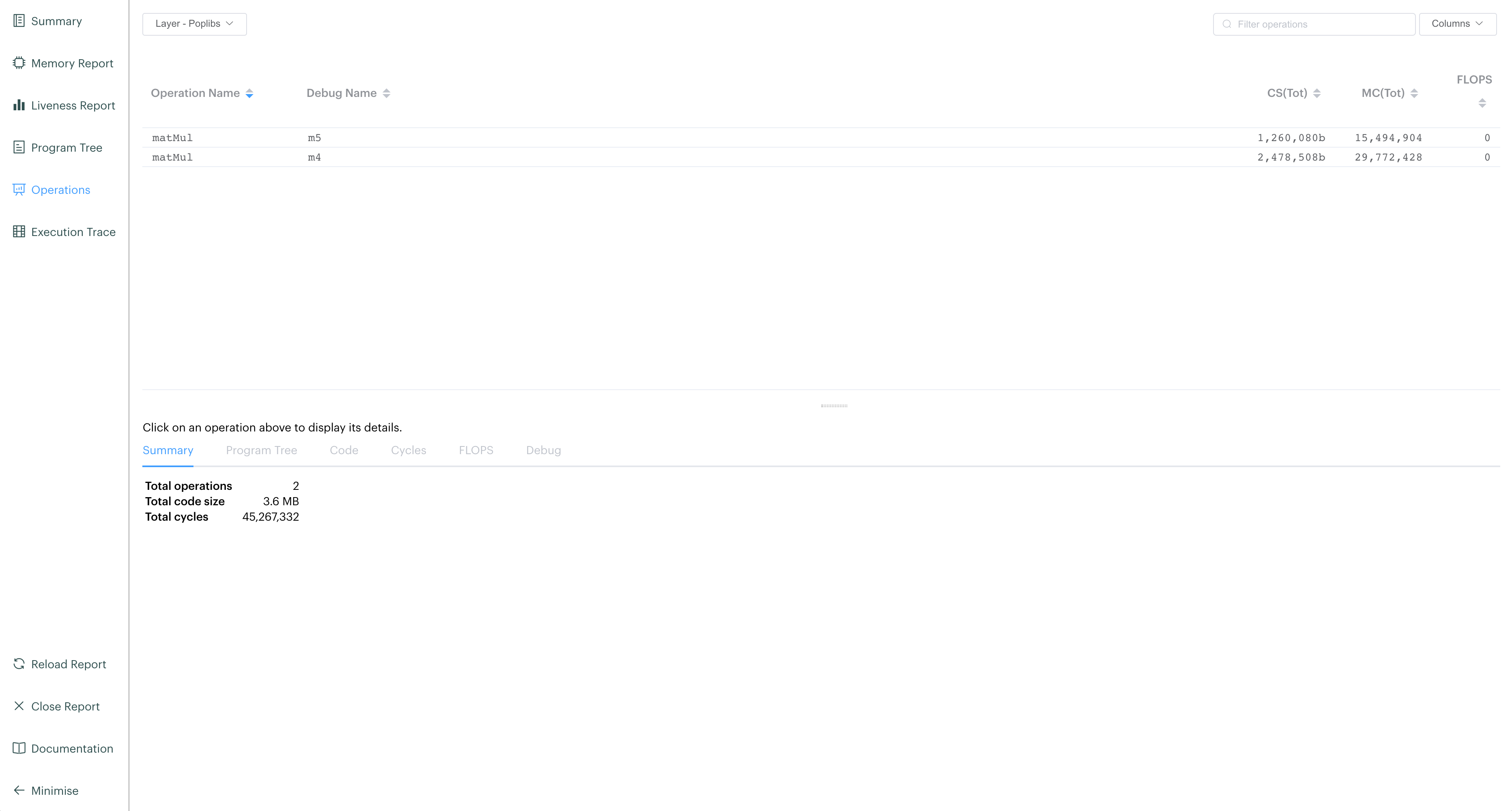
The top panel shows a table listing the operations in the currently selected software layer (the default layer is PopLibs) along with a default set of columns of information.
- The columns displayed can be modified using the Columns drop-down menu in the top-right of the window.
Click on one of the matMul Operations to show the summary for that operation in the bottom panel.
- When no operation is selected this tab shows a breakdown of operations for the selected software.
Click through each tab in the bottom panel (with an operation selected in the top panel):
- Summary - data from the default table columns.
- Program Tree - the program steps involved in the selected operation.
- Code - a graph of the code executed for the selected operation.
- Cycles - the number of cycles taken by the selected operation.
- FLOPS - the number of floating point operations executed for the selected operation.
- Debug - debug information from the selected operation.

More details on Operations and full descriptions of the functionality of each each bottom panel tab are given in the Operations Summary section of the PopVision Graph Analyser documentation.

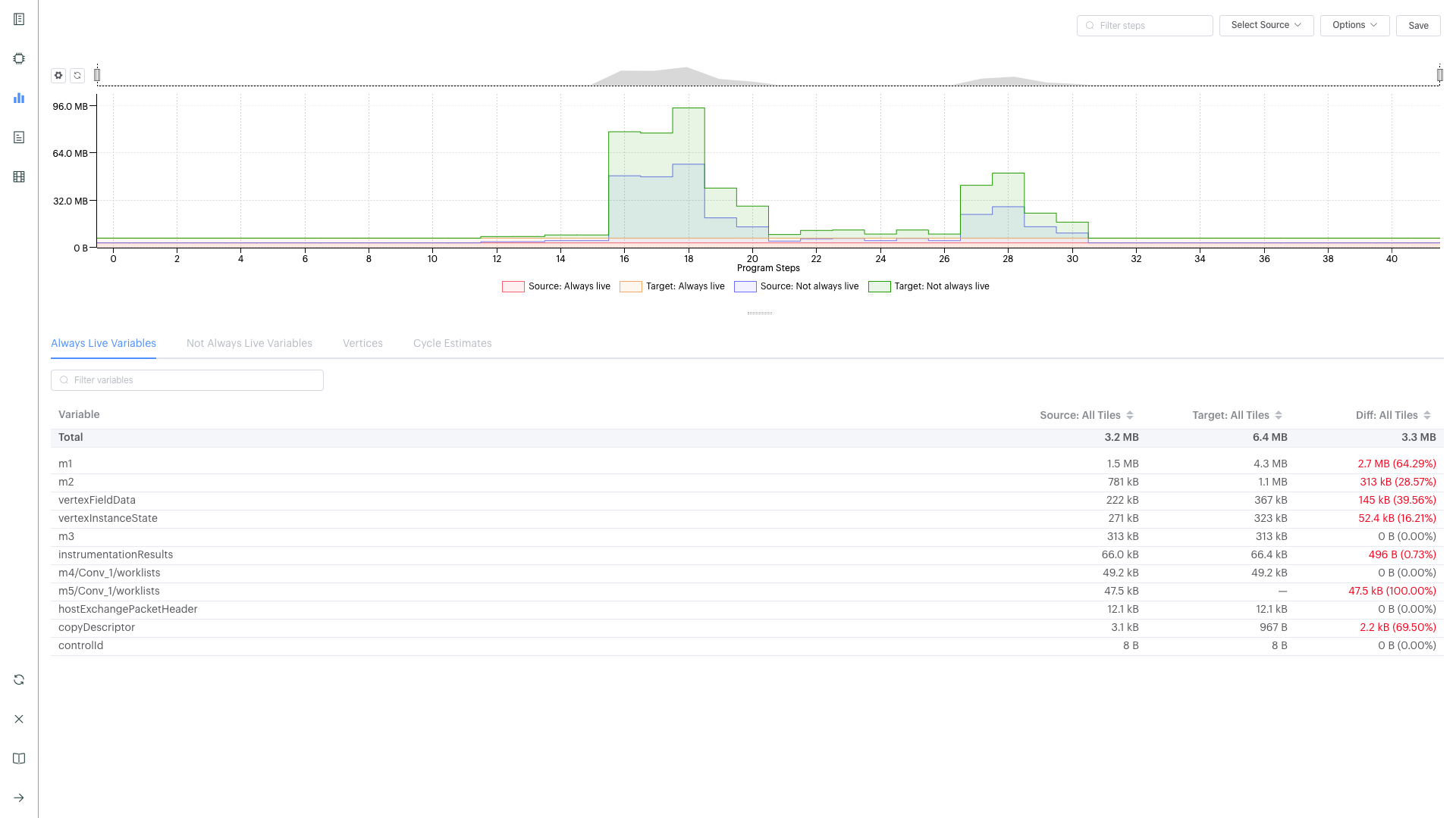
Liveness report

This gives a detailed breakdown of the state of the variables at each step of your program. Some variables persist in memory for the entirety of your program - these are known as ‘Always Live’ variables. Some variables are allocated and deallocated as memory is reused - these are known as ‘Not Always Live’ variables. While the Memory report does track this, the Liveness report visualises it.

Open one of your reports from above, and click on the Liveness Report tab icon on the left.

You should see the Liveness Report tab: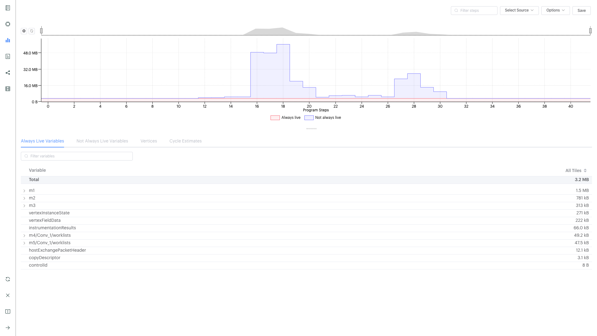
From the Options turn on Include Always Live
Click through different time steps, noting what details are given in the Always Live Variables / Not Always Live Variables / Vertices and Cycle Estimates tabs in the bottom panel.

Note the program steps matching up with the Program Tree.

More details on the Liveness Report are given in the Liveness Report section of the PopVision Graph Analyser documentation.

Execution trace

This shows how many clock cycles each step of an instrumented program consumes. Open one of your reports from above, and click on the Execution Trace tab icon on the left.

You should see the Execution Trace tab:
Switch the Execution View between Flame and Flat, and with BSP on and off.
Observe the sync, exchange and execution code across the tiles.
Observe how these correspond to the different operations, and in the program tree.
Click on the Summary and Details tabs in the lower panel and observe the different information given for different operations.
Note that all the measurements are in clock cycles not time.

More details on the Execution Trace are given in the Execution Trace section of the PopVision Graph Analyser documentation.

Follow-ups

Modify the tutorial code with extra operations and see the effects in the different tabs of PopVision Graph Analyser, or try with your own code.

Summary

In this tutorial, we learnt how to extract useful profiling information from any Poplar program. We first used a method that prints a summary of information on the console, then we learnt how to generate a report by setting an environment variable, and we extracted some information from it using the PopVision analysis API. Finally, we explored in more details the more convenient and easy to use tool for profiling: the PopVision Graph Analyser. In this tutorial we profiled Poplar programs, but using the PopVision Graph Analyser for TensorFlow and PyTorch applications on the IPU is a case of setting the same environment variables. This is described in more details in the PopVision Graph Analyser User Guide.

In the next tutorial you will write a Poplar application that performs matrix-vector multiplication.

To learn more about profiling IPU applications, check also the PopVision tutorials, where you can discover the PopVision System Analyser tool, the PopVision Trace Instrumentation Library (libpvti) and learn more about the PopVision analysis API (libpva), which has been introduced in this tutorial.

For techniques to optimise memory use and improve performance please refer to our memory and performance optimisation guide.

Search help