Source (GitHub) | Download notebook

---

4.1. PopXL and popxl.addons

Introduction

As an alternative to using the ONNX builder to create models, PopXL is an experimental PopART Python module which allows users to hand-craft arbitrary computational graphs, control execution schemes, and optimise the Poplar executable. This provides greater flexibility than is possible using the standard PopART API.

It gives precise control of program size and runtime performance in a high level language (Python). It is useful for large models, as it gives low-level control of:

• Subgraph inlining/outlining for optimising program size

• Data parallelism for improving throughput

• Remote Variables for streaming/storing data remotely to optimise memory requirements of the model

Familiarity with the basic PopXL concepts will be helpful, but not essential:

• Intermediate representation (IR)

• Tensors (variable, constant and intermediate)

• Graphs (main and subgraph)

• Input and output streams

• Sessions

popxl.addons includes common usage patterns of PopXL. It simplifies the process of building and training a model while keeping control of execution and optimisation strategies.

Once you’ve finished this tutorial, you will:

• Be familiar with addons basic concepts and understand relations between them:

  • Module

  • NamedTensors

  • VariableFactory and NamedVariableFactories

  • GraphWithNamedArgs

  • BoundGraph

  • Transforms

• Understand what outlining is and write an outlined model.

• Use addons autodiff transform to obtain the backward graph for your model.

• Write a simple training + test program, copying trained weights from the training session to the test session.

Requirements

1. Install a Poplar SDK (version 2.6 or later) and source the enable.sh scripts for both PopART and Poplar as described in the Getting Started guide for your IPU system.

2. Install system dependencies: apt-get install -y $(< required_apt_packages.txt)

3. Create a Python virtual environment: python3 -m venv <virtual_env>.

4. Activate the virtual environment: . <virtual_env>/bin/activate.

5. Update pip: pip3 install --upgrade pip

6. Install requirements pip3 install -r requirements.txt (this will also install popxl.addons).

python3 -m venv virtual_env
. virtual_env/bin/activate
pip3 install --upgrade pip
pip3 install -r requirements.txt

To run the Jupyter notebook version of this tutorial:

1. Install a Poplar SDK (version 2.6 or later) and source the enable.sh scripts for both PopART and Poplar as described in the Getting Started guide for your IPU system

2. Create a virtual environment

3. In the same virtual environment, install the Jupyter notebook server: python -m pip install jupyter

4. Launch a Jupyter Server on a specific port: jupyter-notebook --no-browser --port <port number>. Be sure to be in the virtual environment.

5. Connect via SSH to your remote machine, forwarding your chosen port: ssh -NL <port number>:localhost:<port number> <your username>@<remote machine>

For more details about this process, or if you need troubleshooting, see our guide on using IPUs from Jupyter notebooks.

If using VS Code, Intellisense can help you understand the tutorial code. It will show function and class descriptions when hovering over their names and lets you easily jump to their definitions. Consult the VSCode setup guide to use Intellisense for this tutorial.

Basic concepts

The following are basic concepts of popxl.addons:

• Module: a module is the base class to build layers and models. It is similar to a PyTorch Module or a Keras Layer. It allows you to create a graph with state, which means with internal parameters (such as weights). Graphs can be called from multiple places in parent graphs, which reduces code duplication.

• NamedTensors : a DotTree collection of popxl.Tensor, which is basically a dictionary between names and tensors. DotTree are used in addons for all collections of named objects. They are very useful to group objects in namespaces.

• VariableFactory and NamedVariableFactories (a DotTree collection of factories): factories are used to delay variable instantiation to the main graph.

• GraphWithNamedArgs: it is a container of a popxl.Graph and NamedTensors. NamedTensors are the graph named inputs. When a GraphWithNamedArgs is created with Module.create_graph(), factories for each of the input tensors are instantiated as well.

• transforms are functions that directly modify the graph, generating a new one. An example is the addons.autodiff transform, which, given a graph, produces the corresponding backward graph.

• BoundGraph: it is a container of a popxl.Graph and a TensorMap of bound Tensor inputs, which are automatically provided as inputs when the graph is called.

The figure below shows how these concepts are related in a typical popxl.addons workflow:

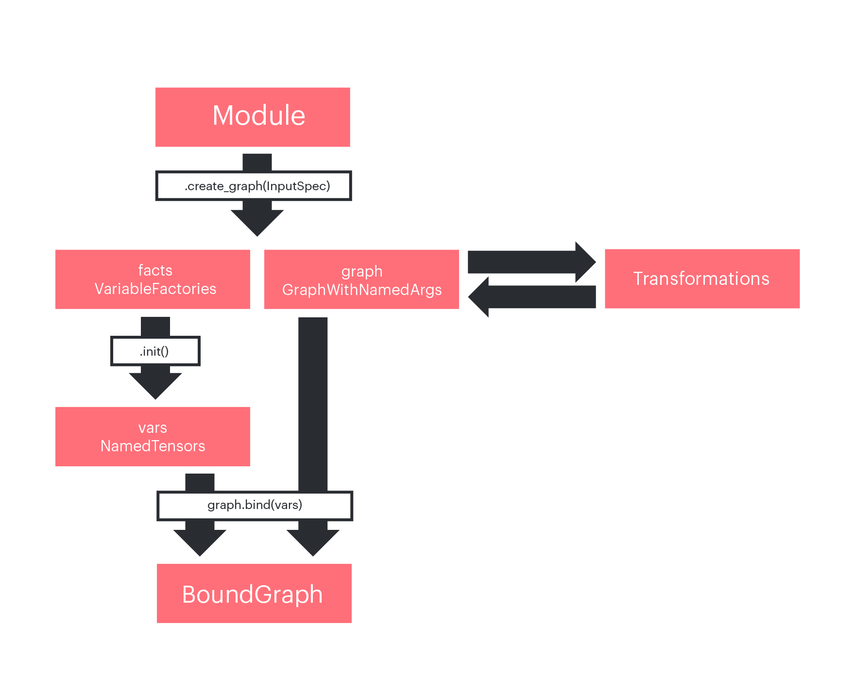
Figure 1: Workflow in popxl.addons.

A simple example

Imports

First let’s import all the packages we are going to need, including popxl and popxl_addons:

from tqdm import tqdm
import torchvision
import torch
import numpy as np
from typing import Mapping, Optional
from functools import partial

np.random.seed(42)

import popxl.ops as ops
import popxl_addons as addons
import popxl

Defining a Linear Module

Below is an example of a linear layer implemented by subclassing addons.Module:

class Linear(addons.Module):
    def __init__(self, out_features: int, bias: bool = True):
        super().__init__()
        self.out_features = out_features
        self.bias = bias

    def build(self, x: popxl.Tensor) -> popxl.Tensor:
        # add a state variable to the module
        w = self.add_variable_input(
            "weight",
            partial(np.random.normal, 0, 0.02, (x.shape[-1], self.out_features)),
            x.dtype,
        )
        y = x @ w
        if self.bias:
            # add a state variable to the module
            b = self.add_variable_input("bias", partial(np.zeros, y.shape[-1]), x.dtype)
            y = y + b

        return y

Each Module needs to implement a build method. Here you actually define the graph, specifying inputs, operations and outputs (the return values).

Inputs are added in two different ways:

• named inputs (the parameters of the model, its state) are added via the add_variable_input method (w and b above).

• All tensor arguments of the build method (x in the example above) become inputs of the graph.

PopXL variables (the parameters of the model) can only live in the main graph which means state tensor variables cannot be instantiated directly in the subgraph; their creation needs to take place in the main graph. The add_variable_input method creates a named local placeholder (a local tensor) and a corresponding VariableFactory. As we will see below, the factory is used to instantiate a variable in the main graph and then bind it to the named input in the subgraph.

Creating a graph from a Module

Before we construct any graphs we need to define a popxl.Ir instance which will hold the main graph. This will represent your fully compiled program.

ir = popxl.Ir(replication=1)

Inside the IR main graph we construct the Linear graph as follows:

with ir.main_graph:
    # create a variable factory and a graph from the module
    facts, linear_graph = Linear(32).create_graph(
        popxl.TensorSpec((2, 4), popxl.float32)
    )
    print("factories: \n", facts)
    print("\n graph: \n", linear_graph.print_schedule())

    # since we are in the main graph, we can instantiate variables using the factories
    variables = facts.init()
    print("\n variables: \n", variables)

    # and bind our graph to these variables that live in the main graph.
    bound_graph = linear_graph.bind(variables)

    # the bound graph can be called providing only unnamed inputs x
    input_data = np.asarray(np.random.rand(2, 4)).astype(np.float32)
    input_tensor = popxl.variable(input_data, name="x")

    out = bound_graph.call(input_tensor)

factories:
 {'weight': <popxl_addons.variable_factory.VariableFactory object at 0x7feaf5cb1160>, 'bias': <popxl_addons.variable_factory.VariableFactory object at 0x7fe851acee10>}

 graph:
 Graph : Linear_subgraph(0)
  (%1, weight=%2, bias=%3) -> (%5) {
    MatMul.100 (%1 [(2, 4) float32], %2 [(4, 32) float32]) -> (%4 [(2, 32) float32])
    Add.101 (%4 [(2, 32) float32], %3 [(32,) float32]) -> (%5 [(2, 32) float32])
  }

 variables:
 {'bias': Tensor[bias popxl.dtypes.float32 (32,)], 'weight': Tensor[weight popxl.dtypes.float32 (4, 32)]}

The create_graph method requires a TensorSpec object or a Tensor object for each of the unnamed inputs (x) and returns a GraphWithNamedArgs and NamedVariableFactories for the named inputs.

The GraphWithNamedArgs gathers together a popxl.Graph and tensors (GraphWithNamedArgs.args) which correspond to the named inputs we added earlier with add_variable_input when we defined the Linear Module.

Also, the NamedVariableFactories collection contains a factory for each of those tensors. Instantiating a variable in the main graph is optional, provided you feed these inputs at the call site. for example linear_graph.call(x,w,b)

Once you have instantiated variables using these factories, you can bind the graph to them using bound_graph = linear_graph.bind(variables).

The resulting BoundGraph is effectively a graph with an internal state, which can be called from the main graph with:

outputs = bound_graph.call(x)

Finally, we specify the properties of the IR and create a session object to run it.

ir.num_host_transfers = 1

# Create a session to run your IR
session = popxl.Session(ir, "ipu_hw")

# Run the program
with session:
    session.run()

Summary and concepts in practice

In summary, the basic steps needed to build and run a model in popxl.addons are the following:

1. Subclass addons.Module to create your layers and models in an object-oriented fashion.

2. Initialise an IR as ir which represents your full compiled program.

3. In the ir.main_graph() context, generate the computational graph and the variable factories associated with your module with the Module create_graph method.

4. In the ir.main_graph() context, instantiate actual variables with the NamedVariableFactory init method.

5. In the ir.main_graph() context, bind the computational graph to the variables using the bind method of GraphWithNamedArgs.

6. In the ir.main_graph() context, call the bound graph providing only the inputs.

7. Specify the properties of the IR and create a popxl.Session to run your IR.

8. Run the program.

Multiple bound graphs

The same subgraph can be bound to different sets of parameters, resulting in different bound graphs. You can think to a bound graph as a container of a graph object and a set of variables. Two different bound graphs can reference to the same graph, but have different variables.

ir = popxl.Ir()
with ir.main_graph:
    facts, linear_graph = Linear(32).create_graph(
        popxl.TensorSpec((2, 4), popxl.float32)
    )

    variables1 = facts.init()
    variables2 = facts.init()

    # the same subgraph can be bound to different variables,
    # generating distinct bound graph objects.
    bound_graph1 = linear_graph.bind(variables1)
    bound_graph2 = linear_graph.bind(variables2)

    print("\n two different bound graphs: \n", bound_graph1, bound_graph2)

    input_data = np.asarray(np.random.rand(2, 4)).astype(np.float32)
    input_tensor = popxl.variable(input_data, name="x")

    out = bound_graph1.call(input_tensor)

 two different bound graphs:
 <popxl_addons.graph.BoundGraph object at 0x7fe851b717b8> <popxl_addons.graph.BoundGraph object at 0x7fe851c3b4a8>

Both bound graphs refer to the same computational graph, hence code is reused on the IPU.

What actually happens is that bound_graph1.call becomes a call operation in the main graph with the following arguments:

call(graph, x, inputs_dict=variables_dict1)

where variables_dict1 is a dictionary between the local tensors in the graph and the corresponding variables in the main graph, created using the factories.

Calling bound_graph2, which is the same graph but bound to different parameters, results in:

call(graph, x, inputs_dict=variables_dict2)

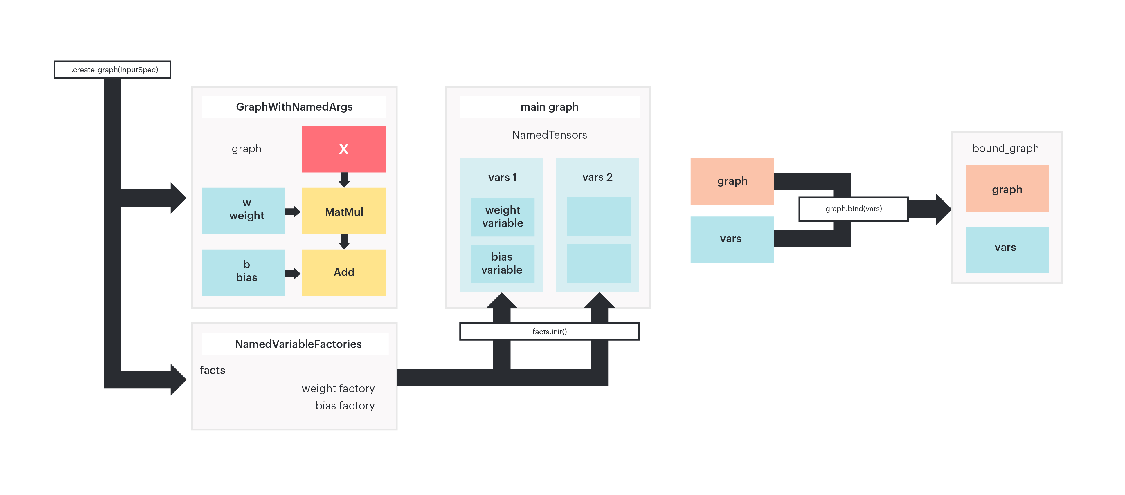
Figure 2: The module.create_graph method generates a graph and named variable factories. Calling .init() on the variable factories instantiates actual variable tensors in the main graph. The same subgraph can be bound to different sets of variables, generating different bound graphs.

Nested Modules and Outlining

Outlining is the opposite of inlining:

• Inlining, which is generally the default behaviour on the IPU means that if a module is used more than once in a model, then a copy will be made of the code on the IPU for each use. This has the effect of better performance, because we remove some of the overhead of calling out to a function, but will use more always-live memory due to code duplication.

• Outlining, conversely requires some explicit PopXL code. Code will only exist once on each IPU and could be called from multiple parent models. This has the effect of reducing total memory requirements at the expense of some performance.

Further information on graph outlining can be found in our memory performance optimisation guide.

These concepts becomes important when we start building more complicated models using the Module api, combining and nesting several modules. To see why, let’s build a simple linear model using several Linear layers.

class Net(addons.Module):
    def __init__(self, cache: Optional[addons.GraphCache] = None):
        super().__init__(cache=cache)
        self.fc1 = Linear(512)
        self.fc2 = Linear(512)
        self.fc3 = Linear(512)
        self.fc4 = Linear(10)

    def build(self, x: popxl.Tensor):
        x = x.reshape((-1, 28 * 28))
        x = ops.gelu(self.fc1(x))
        x = ops.gelu(self.fc2(x))
        x = ops.gelu(self.fc3(x))
        x = self.fc4(x)
        return x


ir = popxl.Ir()
main = ir.main_graph
with main:
    facts, net_graph = Net().create_graph(popxl.TensorSpec((28, 28), popxl.float32))
    print(facts.to_dict().keys())
    print("\n", net_graph.print_schedule())

dict_keys(['fc1.weight', 'fc1.bias', 'fc2.weight', 'fc2.bias', 'fc3.weight', 'fc3.bias', 'fc4.weight', 'fc4.bias'])

 Graph : Net_subgraph(0)
  (%1, fc1.weight=%2, fc1.bias=%3, fc2.weight=%4, fc2.bias=%5, fc3.weight=%6, fc3.bias=%7, fc4.weight=%8, fc4.bias=%9) -> (%21) {
    Reshape.100 (%1 [(28, 28) float32]) -> (%10 [(1, 784) float32])
    MatMul.101 (%10 [(1, 784) float32], %2 [(784, 512) float32]) -> (%11 [(1, 512) float32])
    Add.102 (%11 [(1, 512) float32], %3 [(512,) float32]) -> (%12 [(1, 512) float32])
    Gelu.103 (%12 [(1, 512) float32]) -> (%13 [(1, 512) float32])
    MatMul.104 (%13 [(1, 512) float32], %4 [(512, 512) float32]) -> (%14 [(1, 512) float32])
    Add.105 (%14 [(1, 512) float32], %5 [(512,) float32]) -> (%15 [(1, 512) float32])
    Gelu.106 (%15 [(1, 512) float32]) -> (%16 [(1, 512) float32])
    MatMul.107 (%16 [(1, 512) float32], %6 [(512, 512) float32]) -> (%17 [(1, 512) float32])
    Add.108 (%17 [(1, 512) float32], %7 [(512,) float32]) -> (%18 [(1, 512) float32])
    Gelu.109 (%18 [(1, 512) float32]) -> (%19 [(1, 512) float32])
    MatMul.110 (%19 [(1, 512) float32], %8 [(512, 10) float32]) -> (%20 [(1, 10) float32])
    Add.111 (%20 [(1, 10) float32], %9 [(10,) float32]) -> (%21 [(1, 10) float32])
  }

You can see from the output of print_schedule() that nested modules lead to inlined code: the nodes are repeated for each layer, even if they are identical. For example here fc2 and fc3 have the exact same graph. If you want to achieve better code reuse you can manually outline the graph by explicitly inserting call operations.

To implement outlining using the Module class, you need to:

• Create the graph you want to outline with factories, shared_graph = module.create_graph().

• Generate different named input tensors (different local placeholders) for each layer. To do this, you can use the module.add_variable_inputs(name, factories) method. Every time you call this function, you create distinct local tensors. Moreover, you add factories for these tensors.

• Bind the graph to each set of local tensors, obtaining a different BoundGraph for each layer.

• Add call operations to the bound graphs.

When you call factories.init() in the main context you generate variables for all the local tensors. When you finally bind the graph, the local tensors are bound to the main variables. Since the shared_graph is bound to the local tensors, it is effectively bound to them too.

Below is an outlined version of the network. You can see in the graph that the fc2 and fc3 blocks have been replaced by call operations.

class NetOutlined(addons.Module):
    def __init__(self, cache: Optional[addons.GraphCache] = None):
        super().__init__(cache=cache)
        # first and last layer are not reused
        self.fc1 = Linear(512)
        self.fc4 = Linear(10)

    def build(self, x: popxl.Tensor):
        x = x.reshape((-1, 28 * 28))
        x = ops.gelu(self.fc1(x))

        # create a single subgraph to be used both for fc2 and fc3
        # create variable factories and subgraph
        facts, subgraph = Linear(512).create_graph(x)
        # generate specific named inputs for fc2
        named_tensors_0 = self.add_variable_inputs("fc2", facts)
        # fc2 is a bound graph using the shared, single subgraph and custom params
        fc2 = subgraph.bind(named_tensors_0)
        # generate specific named inputs for fc3
        named_tensors_1 = self.add_variable_inputs("fc3", facts)
        # fc3 is a bound graph using the shared, single subgraph and custom params
        fc3 = subgraph.bind(named_tensors_1)

        (x,) = fc2.call(x)
        x = ops.gelu(x)
        (x,) = fc3.call(x)
        x = ops.gelu(x)

        x = self.fc4(x)
        return x


ir = popxl.Ir()
with ir.main_graph:
    args, net_graph = NetOutlined().create_graph(
        popxl.TensorSpec((28, 28), popxl.float32)
    )
    print(args.to_dict().keys())
    print("\n", net_graph.print_schedule())

dict_keys(['fc1.weight', 'fc1.bias', 'fc4.weight', 'fc4.bias', 'fc2.weight', 'fc2.bias', 'fc3.weight', 'fc3.bias'])

 Graph : NetOutlined_subgraph(0)
  (%1, fc1.weight=%2, fc1.bias=%3, fc2.weight=%4, fc2.bias=%5, fc3.weight=%6, fc3.bias=%7, fc4.weight=%8, fc4.bias=%9) -> (%19) {
    Reshape.100 (%1 [(28, 28) float32]) -> (%10 [(1, 784) float32])
    MatMul.101 (%10 [(1, 784) float32], %2 [(784, 512) float32]) -> (%11 [(1, 512) float32])
    Add.102 (%11 [(1, 512) float32], %3 [(512,) float32]) -> (%12 [(1, 512) float32])
    Gelu.103 (%12 [(1, 512) float32]) -> (%13 [(1, 512) float32])
    Call.106(Linear_subgraph(1)) (%13 [(1, 512) float32], %4 [(512, 512) float32], %5 [(512,) float32]) -> (%14 [(1, 512) float32])
    Gelu.107 (%14 [(1, 512) float32]) -> (%15 [(1, 512) float32])
    Call.108(Linear_subgraph(1)) (%15 [(1, 512) float32], %6 [(512, 512) float32], %7 [(512,) float32]) -> (%16 [(1, 512) float32])
    Gelu.109 (%16 [(1, 512) float32]) -> (%17 [(1, 512) float32])
    MatMul.110 (%17 [(1, 512) float32], %8 [(512, 10) float32]) -> (%18 [(1, 10) float32])
    Add.111 (%18 [(1, 10) float32], %9 [(10,) float32]) -> (%19 [(1, 10) float32])
  }

DotTree example

The following code block is a simple example to help you get familiar with the DotTree syntax used by popxl.addons.

ir = popxl.Ir(replication=1)

with ir.main_graph:
    facts, linear_graph = Linear(32).create_graph(
        popxl.TensorSpec((2, 4), popxl.float32)
    )
    variables = facts.init()
    variables2 = facts.init()

    print("----- DotTree functionalities -----\n")
    collection = addons.NamedTensors()  # empty collection
    collection.insert("layer1", variables)  # add a new key with the insert method
    collection.insert("layer2", variables2)
    print(
        "A nested collection: the nested structure appear from the dot structure of names"
    )
    print(collection, "\n")  # nested structure
    print("Each leaf can be accessed with dot syntax: collection.layer1")
    print(
        collection.layer1
    )  # each leaf node in the tree can be accessed with dot syntax
    collection_dict = collection.to_dict()  # convert the collection to dictionary

    nt = addons.NamedTensors.from_dict(
        {"x": input_tensor}
    )  # create the collection from a dictionary
    nt_b = addons.NamedTensors.from_dict({"b": variables.bias})
    nt.update(
        nt_b
    )  # update the collection with another collection, keys should not repeat
    # print("\n",nt)

    names = ["new_bias_name", "new_weight_name"]
    nt_from_lists = addons.NamedTensors.pack(
        names, variables.tensors
    )  # create the collection from a list
    names, tensors = nt_from_lists.unpack()
    # print("\n",nt_from_lists)

    print("\n")

    # ----- NamedTensors specific -----
    print("----- NamedTensors -----\n")
    print(collection.named_tensors, "\n")  # same as to_dict, specific of NamedTensors
    print("Get only tensors, sorted by name")
    print(collection.tensors)  # returns tensors, sorted by names

----- DotTree functionalities -----

A nested collection: the nested structure appear from the dot structure of names
{'layer1.bias': Tensor[bias popxl.dtypes.float32 (32,)], 'layer1.weight': Tensor[weight popxl.dtypes.float32 (4, 32)], 'layer2.bias': Tensor[bias__t0 popxl.dtypes.float32 (32,)], 'layer2.weight': Tensor[weight__t1 popxl.dtypes.float32 (4, 32)]}

Each leaf can be accessed with dot syntax: collection.layer1
{'bias': Tensor[bias popxl.dtypes.float32 (32,)], 'weight': Tensor[weight popxl.dtypes.float32 (4, 32)]}


----- NamedTensors -----

{'layer1.bias': Tensor[bias popxl.dtypes.float32 (32,)], 'layer1.weight': Tensor[weight popxl.dtypes.float32 (4, 32)], 'layer2.bias': Tensor[bias__t0 popxl.dtypes.float32 (32,)], 'layer2.weight': Tensor[weight__t1 popxl.dtypes.float32 (4, 32)]}

Get only tensors, sorted by name
(Tensor[bias popxl.dtypes.float32 (32,)], Tensor[bias__t0 popxl.dtypes.float32 (32,)], Tensor[weight popxl.dtypes.float32 (4, 32)], Tensor[weight__t1 popxl.dtypes.float32 (4, 32)])

You can experiment with the above code to explore the api before going through the full MNIST program.

MNIST

Load dataset

We are now ready to build the full program to train and validate a linear model on the MNIST dataset.

First of all, we need to load the dataset. We are going to use a PyTorch DataLoader. Data is normalised using the mean and std deviation of the dataset.

def get_mnist_data(test_batch_size: int, batch_size: int):
    training_data = torch.utils.data.DataLoader(
        torchvision.datasets.MNIST(
            "~/.torch/datasets",
            train=True,
            download=True,
            transform=torchvision.transforms.Compose(
                [
                    torchvision.transforms.ToTensor(),
                    # mean and std computed on the training set.
                    torchvision.transforms.Normalize((0.1307,), (0.3081,)),
                ]
            ),
        ),
        batch_size=batch_size,
        shuffle=True,
        drop_last=True,
    )

    validation_data = torch.utils.data.DataLoader(
        torchvision.datasets.MNIST(
            "~/.torch/datasets",
            train=False,
            download=True,
            transform=torchvision.transforms.Compose(
                [
                    torchvision.transforms.ToTensor(),
                    torchvision.transforms.Normalize((0.1307,), (0.3081,)),
                ]
            ),
        ),
        batch_size=test_batch_size,
        shuffle=True,
        drop_last=True,
    )

    return training_data, validation_data

Defining the Training step

Now that we have a dataset and a model we are ready to construct the training program.

First of all let’s define a function to build the training program.

def train_program(batch_size, device, learning_rate):
    ir = popxl.Ir(replication=1)

    with ir.main_graph:
        # Create input streams from host to device
        img_stream = popxl.h2d_stream((batch_size, 28, 28), popxl.float32, "image")
        img_t = ops.host_load(img_stream)  # load data
        label_stream = popxl.h2d_stream((batch_size,), popxl.int32, "labels")
        labels = ops.host_load(label_stream, "labels")

        # Create forward graph
        facts, fwd_graph = Net().create_graph(img_t)
        # Create backward graph via autodiff transform
        bwd_graph = addons.autodiff(fwd_graph)

        # Initialise variables (weights)
        variables = facts.init()

        # Call the forward graph with call_with_info because we want to retrieve
        # information from the call site
        fwd_info = fwd_graph.bind(variables).call_with_info(img_t)
        x = fwd_info.outputs[0]  # forward output

        # Compute loss and starting gradient for backpropagation
        loss, dx = addons.ops.cross_entropy_with_grad(x, labels)

        # Setup a stream to retrieve loss values from the host
        loss_stream = popxl.d2h_stream(loss.shape, loss.dtype, "loss")
        ops.host_store(loss_stream, loss)

        # retrieve activations from the forward graph
        activations = bwd_graph.grad_graph_info.inputs_dict(fwd_info)
        # call the backward graph providing the starting value for backpropagation and activations
        bwd_info = bwd_graph.call_with_info(dx, args=activations)

        # Optimiser: get a mapping between forward tensors and corresponding
        # gradients and use it to update each tensor
        grads_dict = bwd_graph.grad_graph_info.fwd_parent_ins_to_grad_parent_outs(
            fwd_info, bwd_info
        )
        for t in variables.tensors:
            ops.scaled_add_(t, grads_dict[t], b=-learning_rate)

    ir.num_host_transfers = 1
    return popxl.Session(ir, device), [img_stream, label_stream], variables, loss_stream

We need to specify the replication_factor for the IR before constructing the program, because some operations need to know the number of IPUs involved.

Inside the main graph context of the IR, we construct streams to transfer input data from the host to the device (popxl.h2d_stream) and we load data to the device (popxl.host_load).

Then, we create two graphs: one for the forward pass and one for the backward pass. The latter can be obtained from the forward graph applying a transform, which is a way of making changes at the graph level. The addons.autodiff transform is the one we need. It is basically popxl.autodiff with some additional patterns.

We instantiate the weights of the network (variables = facts.init()), bind the forward graph to these variables and make the call to the forward graph. We use call_with_info because we want to be able to retrieve the activations from the forward graph and pass them to the backward graph (see calling-a-subgraph)

The cross_entropy_with_grad operation returns the loss tensor and the gradient to start backpropagation, which is 1 (dl/dl) unless you specify the additional argument loss_scaling.

We create an output stream from the device to the host in order to retrieve loss values.

We call the backward graph and retrieve a dictionary mapping each tensor in the forward graph to its corresponding gradient in the backward graph with fwd_parent_ins_to_grad_parent_outs. This dictionary can then be used by the optimiser to update the weights of the model.

Finally, we setup the properties for ir, specifying num_host_transfers, and we return a popxl.Session so that we can execute our program.

Now we are ready to construct the model using the following hyper-parameters:

train_batch_size = 8
test_batch_size = 80
device = "ipu_hw"
learning_rate = 0.05
epochs = 1

training_data, test_data = get_mnist_data(test_batch_size, train_batch_size)

train_session, train_input_streams, train_variables, loss_stream = train_program(
    train_batch_size, device, learning_rate
)

And train it as follows:

num_batches = len(training_data)
with train_session:
    for epoch in range(1, epochs + 1):
        print(f"Epoch {epoch}/{epochs}")
        bar = tqdm(training_data, total=num_batches)
        for data, labels in bar:
            inputs: Mapping[popxl.HostToDeviceStream, np.ndarray] = dict(
                zip(train_input_streams, [data.squeeze().float(), labels.int()])
            )
            loss = train_session.run(inputs)[loss_stream]
            bar.set_description(f"Loss:{loss:0.4f}")

Epoch 1/1
Loss:0.0270: 100%|██████████| 7500/7500 [00:24<00:00, 306.92it/s]

After training we retrieve the trained weights to use them during inference and test the accuracy of the model. To do that, we need to get the data stored in the tensor on the device with get_tensors_data.

train_vars_to_data = train_session.get_tensors_data(train_variables.tensors)

Validation

To test our model we need to create an inference-only program and run it on the test dataset.

def test_program(test_batch_size, device):
    ir = popxl.Ir(replication=1)

    with ir.main_graph:
        # Inputs
        in_stream = popxl.h2d_stream((test_batch_size, 28, 28), popxl.float32, "image")
        in_t = ops.host_load(in_stream)

        # Create graphs
        facts, graph = Net().create_graph(in_t)

        # Initialise variables
        variables = facts.init()

        # Forward
        (outputs,) = graph.bind(variables).call(in_t)
        out_stream = popxl.d2h_stream(outputs.shape, outputs.dtype, "outputs")
        ops.host_store(out_stream, outputs)

    ir.num_host_transfers = 1
    return popxl.Session(ir, device), [in_stream], variables, out_stream

Again, we initialise the IR. Then, we define the input stream, the graph and the factories for the variables. We instantiate the variables and bind the graph to them, obtaining our bound graph. Finally, we call the model. Since this time we do not need to retrieve information from the call site, we can simply use call instead of call_with_info. We store the output in an output stream for later use.

We now call the function to create the test program and initialise the session:

test_session, test_input_streams, test_variables, out_stream = test_program(
    test_batch_size, device
)

Before we run, we need to initialise the model variables with the weights we trained earlier.

To do that, once the test_session is created we can call test_session.write_variables_data. This function requires a dictionary tensor_to_be_written : tensor_data_to_write. It makes a call to test_session.write_variable_data(tensor,tensor_data) for each tensor in the dictionary and then makes a single host to device transfer at the end to send all data in one go. In our case, tensor_to_be_written needs to be the test_session variables, and tensor_data_to_write needs to be the tensor values, given as numpy arrays.

We already have a dictionary between train_session variables and their values, the train_weights_data_dict retrieved with train_session.get_tensor_data.

We need a dictionary between the test_session variables and the train_session variables, so that we can create the required test_variables : test_variables_data dictionary.

Provided test and training variables have the same names, we can use the DotTree.to_mapping function to create this mapping. Given two DotTrees, for common keys this function creates a dictionary of their values. So, train_variables.to_mapping(test_variables) returns a dictionary popxl.Tensor : popxl.Tensor, where each key-value pair is made of a train variable and the test variable with the same name.

With these two dictionaries, we can finally build the required test_variables : test_variables_data dictionary.

Earlier we saved the trained weights to train_vars_to_data.

# dictionary { train_session variables : test_session variables }
train_vars_to_test_vars = train_variables.to_mapping(test_variables)

# Create a dictionary { test_session variables : tensor data (numpy) }
test_vars_to_data = {
    test_var: train_vars_to_data[train_var].copy()
    for train_var, test_var in train_vars_to_test_vars.items()
}

We call .copy on each tensor because get_tensors_data returns a memory view of the data. This may become invalid if the session is invalidated (or it may change if we do something else later).

# Copy trained weights to the program, with a single host to device transfer
test_session.write_variables_data(test_vars_to_data)

# check that weights have been copied correctly
test_vars_to_data_after_write = test_session.get_tensors_data(test_variables.tensors)
for test_var, array in test_vars_to_data_after_write.items():
    assert (array == test_vars_to_data[test_var]).all()

Finally, we can run the model and evaluate accuracy from the predictions of the model. The predictions do not need to be normalized.

def accuracy(predictions: np.ndarray, labels: np.ndarray):
    ind = np.argmax(predictions, axis=-1).flatten()
    labels = labels.detach().numpy().flatten()
    return np.mean(ind == labels) * 100.0


num_batches = len(test_data)
sum_acc = 0.0
with test_session:
    for data, labels in tqdm(test_data, total=num_batches):
        inputs: Mapping[popxl.HostToDeviceStream, np.ndarray] = dict(
            zip(test_input_streams, [data.squeeze().float(), labels.int()])
        )
        output = test_session.run(inputs)
        sum_acc += accuracy(output[out_stream], labels)

test_set_accuracy = sum_acc / len(test_data)
print(f"Accuracy on test set: {test_set_accuracy:0.2f}%")

100%|██████████| 125/125 [00:01<00:00, 95.71it/s]Accuracy on test set: 96.16%

Conclusion

In this tutorial we explored the new PopXL API. We achieved the following:

• built a simple Linear model (by subclassing addons.Module) and ran it.

• created a multi-layer model with subgraphs and explored outlining. Outlining reduces program size by compiling subgraphs as callable functions rather than inlined code. We constructed subgraphs using create_graph() and bound them explicitly to make 2 layers of a network.

• explored the DotTree syntax which is useful for accessing elements of the model and creating connections.

• built and trained a full MNIST model. The gradients were calculated with the addons.autodiff transform applied to the forward computational graph.

We will re-use the addons.Module class, in another tutorial, when we make a custom optimiser.

To try out more features in PopXL look at our other tutorials.

You can also read our PopXL User Guide for more information.

As the PopXL API is still experimental, we would love to hear your feedback on it (support@graphcore.ai). Your input could help drive its future direction.

Generated:2022-07-22T13:03 Source:mnist.py SDK:2.6.0+1074 SST:0.0.7