2.4. Half and mixed precision in PopTorch

This tutorial shows how to use half and mixed precision in PopTorch with the example task of training a simple CNN model on a single Graphcore IPU (Mk1 or Mk2).

Before starting this tutorial, we recommend that you read through our tutorial on the basics of PyTorch on the IPU and our MNIST starting tutorial.

Requirements:

A Poplar SDK environment enabled (see the Getting Started guide for your IPU system)
Other Python modules: python -m pip install -r requirements.txt

To run the Jupyter notebook version of this tutorial:

Enable a Poplar SDK environment and install required packages with python -m pip install -r requirements.txt;
In the same environment, install the Jupyter notebook server: python -m pip install jupyter;
Launch a Jupyter Server on a specific port: jupyter-notebook --no-browser --port <port number>;
Connect via SSH to your remote machine, forwarding your chosen port: ssh -NL <port number>:localhost:<port number> <your username>@<remote machine>.

For more details about this process, or if you need troubleshooting, see our guide on using IPUs from Jupyter notebooks.

General

Motives for half precision

Data is stored in memory, and some formats to store that data require less memory than others. In a device’s memory, when it comes to numerical data, we use either integers or real numbers. Real numbers are represented by one of several floating point formats, which vary in how many bits they use to represent each number. Using more bits allows for greater precision and a wider range of representable numbers, whereas using fewer bits allows for faster calculations and reduces memory and power usage.

In deep learning applications, where less precise calculations are acceptable and throughput is critical, using a lower precision format can provide substantial gains in performance.

The Graphcore IPU provides native support for two floating-point formats:

IEEE single-precision, which uses 32 bits for each number (FP32)
IEEE half-precision, which uses 16 bits for each number (FP16)

Some applications which use FP16 do all calculations in FP16, whereas others use a mix of FP16 and FP32. The latter approach is known as mixed precision.

In this tutorial, we are going to talk about real numbers represented in FP32 and FP16, and how to use these data types (dtypes) in PopTorch in order to reduce the memory requirements of a model.

Numerical stability

Numeric stability refers to how a model’s performance is affected by the use of a lower-precision dtype. We say an operation is “numerically unstable” in FP16 if running it in this dtype causes the model to have worse accuracy compared to running the operation in FP32. Two techniques that can be used to increase the numerical stability of a model are loss scaling and stochastic rounding.

Loss scaling

A numerical issue that can occur when training a model in half-precision is that the gradients can underflow. This can be difficult to debug because the model will simply appear to not be training, and can be especially damaging because any gradients which underflow will propagate a value of 0 backwards to other gradient calculations.

The standard solution to this is known as loss scaling, which consists of scaling up the loss value right before the start of backpropagation to prevent numerical underflow of the gradients. Instructions on how to use loss scaling will be discussed later in this tutorial.

Stochastic rounding

When training in half or mixed precision, numbers multiplied by each other will need to be rounded in order to fit into the floating point format used. Stochastic rounding is the process of using a probabilistic equation for the rounding. Instead of always rounding to the nearest representable number, we round up or down with a probability such that the expected value after rounding is equal to the value before rounding. Since the expected value of an addition after rounding is equal to the exact result of the addition, the expected value of a sum is also its exact value.

This means that on average, the values of the parameters of a network will be close to the values they would have had if a higher-precision format had been used. The added bonus of using stochastic rounding is that the parameters can be stored in FP16, which means the parameters can be stored using half as much memory. This can be especially helpful when training with small batch sizes, where the memory used to store the parameters is proportionally greater than the memory used to store parameters when training with large batch sizes.

It is highly recommended that you enable this feature when training neural networks with FP16 weights. The instructions to enable it in PopTorch are presented later in this tutorial.

Train a model in half precision

Import the packages

import torch
import torch.nn as nn
import torchvision
import torchvision.transforms as transforms
import poptorch
from tqdm import tqdm

Build the model

We use the same model as in the other tutorials on PopTorch. Just like in the tutorial on efficient data loading, we are using larger images (128x128) to simulate a heavier data load. This will make the difference in memory between FP32 and FP16 meaningful enough to showcase in this tutorial.

class CustomModel(nn.Module):
    def __init__(self):
        super().__init__()
        self.conv1 = nn.Conv2d(1, 5, 3)
        self.pool = nn.MaxPool2d(2, 2)
        self.conv2 = nn.Conv2d(5, 12, 5)
        self.norm = nn.GroupNorm(3, 12)
        self.fc1 = nn.Linear(41772, 100)
        self.relu = nn.ReLU()
        self.fc2 = nn.Linear(100, 10)
        self.log_softmax = nn.LogSoftmax(dim=0)
        self.loss = nn.NLLLoss()

    def forward(self, x, labels=None):
        x = self.pool(self.relu(self.conv1(x)))
        x = self.norm(self.relu(self.conv2(x)))
        x = torch.flatten(x, start_dim=1)
        x = self.relu(self.fc1(x))
        x = self.log_softmax(self.fc2(x))
        # The model is responsible for the calculation
        # of the loss when using an IPU. We do it this way:
        if self.training:
            return x, self.loss(x, labels)
        return x

NOTE: The model inherits self.training from torch.nn.Module which initialises its value to True. Use model.eval() to set it to False and model.train() to switch it back to True.

Choose parameters

NOTE: If you wish to modify these parameters for educational purposes, make sure you re-run all the cells below this one, including this entire cell as well:

# Cast the model parameters and data to FP16
execution_half = True

# Cast the accumulation of gradients values types of the optimiser to FP16
optimizer_half = True

# Use stochastic rounding
stochastic_rounding = True

# Set partials data type to FP16
partials_half = False

Casting a model’s parameters

The default data type of the parameters of a PyTorch module is FP32 (torch.float32). To convert all the parameters of a model to be represented in FP16 (torch.float16), an operation we will call downcasting, we simply do:

model = CustomModel()

if execution_half:
    model = model.half()

For this tutorial, we will cast all the model’s parameters to FP16.

Casting a single layer’s parameters

For bigger or more complex models, downcasting all the layers may generate numerical instabilities and cause underflows. While the PopTorch and the IPU offer features to alleviate those issues, it is still sensible for those models to cast only the parameters of certain layers and observe how it affects the overall training job. To downcast the parameters of a single layer, we select the layer by its name and use half():

model.conv1 = model.conv1.half()

If you would like to upcast a layer instead, you can use model.conv1.float().

NOTE: One can print out a list of the components of a PyTorch model, with their names, by doing print(model).

Prepare the data

We will use the FashionMNIST dataset that we download from torchvision. The last stage of the pipeline will have to convert the data type of the tensors representing the images to torch.half (equivalent to torch.float16) so that our input data is also in FP16. This has the advantage of reducing the bandwidth needed between the host and the IPU.

transform_list = [
    transforms.Resize(128),
    transforms.ToTensor(),
    transforms.Normalize((0.5,), (0.5,)),
]
if execution_half:
    transform_list.append(transforms.ConvertImageDtype(torch.half))

transform = transforms.Compose(transform_list)

Pull the datasets if they are not available locally:

train_dataset = torchvision.datasets.FashionMNIST(
    "~/.torch/datasets", transform=transform, download=True, train=True
)
test_dataset = torchvision.datasets.FashionMNIST(
    "~/.torch/datasets", transform=transform, download=True, train=False
)

Optimizers and loss scaling

The value of the loss scaling factor can be passed as a parameter to the optimisers in poptorch.optim. In this tutorial, we will set it to 1024 for an AdamW optimizer. For all optimisers (except poptorch.optim.SGD), using a model in FP16 requires the argument accum_type to be set to torch.float16 as well:

accum, loss_scaling = (torch.float16, 1024) if optimizer_half else (torch.float32, None)

optimizer = poptorch.optim.AdamW(
    params=model.parameters(), lr=0.001, accum_type=accum, loss_scaling=loss_scaling
)

While higher values of loss_scaling minimize underflows, values that are too high can also generate overflows as well as hurt convergence of the loss. The optimal value depends on the model and the training job. This is therefore a hyperparameter for you to tune.

Set PopTorch’s options

To configure some features of the IPU and to be able to use PopTorch’s classes in the next sections, we will need to create an instance of poptorch.Options which stores the options we will be using. We covered some of the available options in the: introductory tutorial for PopTorch.

Let’s initialise our options object before we talk about the options we will use:

opts = poptorch.Options()

NOTE: This tutorial has been designed to be run on a single IPU. If you do not have access to an IPU, you can use the option useIpuModel to run a simulation on CPU instead. You can read more on the IPU Model and its limitations here.

Stochastic rounding on IPU

With the IPU, stochastic rounding is implemented directly in the hardware and only requires you to enable it. To do so, there is the option enableStochasticRounding in the Precision namespace of poptorch.Options. This namespace holds other options for using mixed precision that we will talk about. To enable stochastic rounding, we do:

if stochastic_rounding:
    opts.Precision.enableStochasticRounding(True)

With the IPU Model, this option won’t change anything since stochastic rounding is implemented on the IPU.

Partials data type

Matrix multiplications and convolutions have intermediate states we call partials. Those partials can be stored in FP32 or FP16. There is a memory benefit to using FP16 partials but the main benefit is that it can increase the throughput for some models without affecting accuracy. However there is a risk of increasing numerical instability if the values being multiplied are small, due to underflows. The default data type of partials is the input’s data type (FP16). For this tutorial, we set partials to FP32 just to showcase how it can be done. We use the option setPartialsType to do it:

if partials_half:
    opts.Precision.setPartialsType(torch.half)
else:
    opts.Precision.setPartialsType(torch.float)

Further information on the Partials Type setting can be found in our memory and performance optimisation guide.

Train the model

We can now train the model. After we have set all our options, we reuse our poptorch.Options instance for the training poptorch.DataLoader that we will be using:

train_dataloader = poptorch.DataLoader(
    opts, train_dataset, batch_size=12, shuffle=True, num_workers=40
)

We first make sure our model is in training mode, and then wrap it with poptorch.trainingModel:

model.train()  # Switch the model to training mode
poptorch_model = poptorch.trainingModel(model, options=opts, optimizer=optimizer)

Let’s run the training loop for 10 epochs:

epochs = 10
for epoch in tqdm(range(epochs), desc="epochs"):
    total_loss = 0.0
    for data, labels in tqdm(train_dataloader, desc="batches", leave=False):
        output, loss = poptorch_model(data, labels)
        total_loss += loss

… and release IPU resources:

poptorch_model.detachFromDevice()

Our new model is now trained and we can start its evaluation.

Evaluate the model

Some PyTorch’s operations, such as CNNs, are not supported in FP16 on the CPU, so we will evaluate our fine-tuned model in mixed precision on an IPU using poptorch.inferenceModel:

model.eval()  # Switch the model to inference mode
poptorch_model_inf = poptorch.inferenceModel(model, options=opts)
test_dataloader = poptorch.DataLoader(opts, test_dataset, batch_size=32, num_workers=40)

Run inference on the labelled data:

predictions, labels = [], []
for data, label in test_dataloader:
    predictions += poptorch_model_inf(data).data.float().max(dim=1).indices
    labels += label

Release resources:

poptorch_model_inf.detachFromDevice()

We obtained an accuracy of approximately 84% on the test dataset.

print(
    f"""Eval accuracy on IPU: {100 *
                (1 - torch.count_nonzero(torch.sub(torch.tensor(labels),
                torch.tensor(predictions))) / len(labels)):.2f}%"""
)

Visualise the memory footprint

We can visually compare the memory footprint on the IPU of the model trained in FP16 and FP32, thanks to Graphcore’s PopVision Graph Analyser.

We generated memory reports of the same training session as covered in this tutorial for both cases: with and without downcasting the model with model.half(). Here is the figure of both memory footprints, where “source” and “target” represent the model trained in FP16 and FP32 respectively:

Comparison of memory footprints

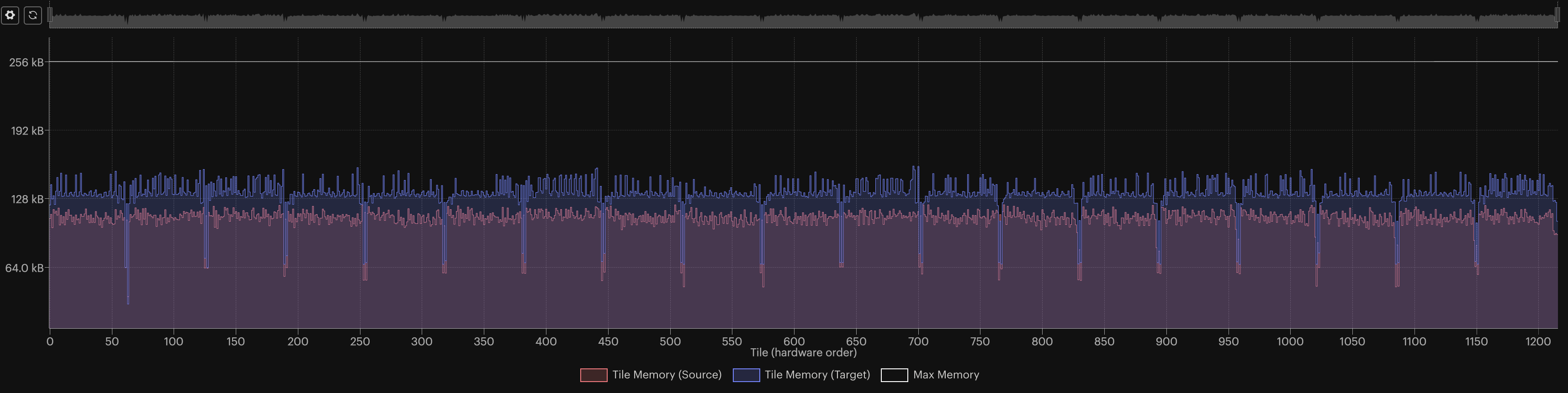
We observed a ~26% reduction in memory usage with the settings of this tutorial, including from peak to peak. The impact on the accuracy was also small, with less than 1% lost!

Debug floating-point exceptions

Floating-point issues can be difficult to debug because the model will simply appear to not be training without specific information about what went wrong. For more detailed information on the issue we set debug.floatPointOpException to true in the environment variable POPLAR_ENGINE_OPTIONS. To set this, you can add the following before the command you use to run your model:

POPLAR_ENGINE_OPTIONS = '{"debug.floatPointOpException": "true"}'

Summary

Use half and mixed precision when you need to save memory on the IPU;
You can cast a PyTorch model or a specific layer to FP16 using:
```
# Model
model.half()
# Layer
model.layer.half()
```
Several features are available in PopTorch to improve the numerical stability of a model in FP16:
- Loss scaling: poptorch.optim.SGD(..., loss_scaling=1000);
- Stochastic rounding: opts.Precision.enableStochasticRounding(True);
- Upcast partials data types: opts.Precision.setPartialsType(torch.float)
The PopVision Graph Analyser can be used to inspect the memory usage of a model and to help debug issues.

Generated:2022-11-22T13:37 Source:walkthrough.py SDK:3.1.0-EA.1+1183 SST:0.0.9

Search help