Source (GitHub) | Download notebook

---

2.1. Introduction to PopTorch - running a simple model

This tutorial covers the basics of model making in PyTorch, using torch.nn.Module, and the specific methods to convert a PyTorch model to a PopTorch model so that it can be run on a Graphcore IPU.

To run the Python version of this tutorial:

1. Download and install the Poplar SDK. Run the enable.sh scripts for Poplar and PopART as described in the Getting Started guide for your IPU system.

2. For repeatability we recommend that you create and activate a Python virtual environment. You can do this with: a. create a virtual environment in the directory venv: virtualenv -p python3 venv; b. activate it: source venv/bin/activate.

3. Install the Python packages that this tutorial needs with python -m pip install -r requirements.txt.

To run the Jupyter notebook version of this tutorial:

1. Enable a Poplar SDK environment (see the Getting Started guide for your IPU system)

2. In the same environment, install the Jupyter notebook server: python -m pip install jupyter

3. Launch a Jupyter Server on a specific port: jupyter-notebook --no-browser --port <port number>

4. Connect via SSH to your remote machine, forwarding your chosen port: ssh -NL <port number>:localhost:<port number> <your username>@<remote machine>

For more details about this process, or if you need troubleshooting, see our guide on using IPUs from Jupyter notebooks.

What is PopTorch?

PopTorch is a set of extensions for PyTorch to enable PyTorch models to run on Graphcore’s IPU hardware.

PopTorch supports both inference and training. To run a model on the IPU you wrap your existing PyTorch model in either a PopTorch inference wrapper or a PopTorch training wrapper. You can provide further annotations to partition the model across multiple IPUs.

You can wrap individual layers in an IPU helper to designate which IPU they should go on. Using your annotations, PopTorch will use PopART to parallelise the model over the given number of IPUs. Additional parallelism can be expressed via a replication factor which enables you to data-parallelise the model over more IPUs.

Under the hood PopTorch uses TorchScript, an intermediate representation (IR) of a PyTorch model, using the torch.jit.trace API. That means it inherits the constraints of that API. These include:

• Inputs must be Torch tensors or tuples/lists containing Torch tensors

• None can be used as a default value for a parameter but cannot be explicitly passed as an input value

• Hooks and .grad cannot be used to inspect weights and gradients

• torch.jit.trace cannot handle control flow or shape variations within the model. That is, the inputs passed at run-time cannot vary the control flow of the model or the shapes/sizes of results.

To learn more about TorchScript and JIT, you can go through the Introduction to TorchScript tutorial.

PopTorch has been designed to require only a few manual changes to your models in order to run them on the IPU. However, it does have some differences from native PyTorch execution and not all PyTorch operations have been implemented in the backend yet. You can find the list of supported operations in the here.

Getting started: training a model on the IPU

We will do the following steps in order:

1. Load the Fashion-MNIST dataset using torchvision.datasets and poptorch.DataLoader.

2. Define a deep CNN and a loss function using the torch API.

3. Train the model on an IPU using poptorch.trainingModel.

4. Evaluate the model on the IPU.

Import the packages

PopTorch is a separate package from PyTorch, and available in Graphcore’s Poplar SDK. Both must thus be imported:

import torch
import poptorch
import torchvision
import torch.nn as nn
import matplotlib.pyplot as plt
from tqdm import tqdm

# Set torch random seed for reproducibility
torch.manual_seed(42)

Under the hood, PopTorch uses Graphcore’s high-performance machine learning framework PopART. It is therefore necessary to enable PopART and Poplar in your environment.

NOTE:

If you forget to enable PopART, you will encounter the following error when importing: poptorch: ImportError: libpopart.so: cannot open shared object file: No such file or directory

If the error message says something like: libpopart_compiler.so: undefined symbol: _ZN6popart7Session3runERNS_7IStepIOE, it most likely means the versions of PopART and PopTorch do not match, for example because you have sourced the PopART enable.sh script for a different SDK version to that of PopTorch. Ensure that you use the same version of the SDK for PopTorch and PopART.

Load the data

We will use the Fashion-MNIST dataset made available by the package torchvision. This dataset, from Zalando, can be used as a more challenging replacement to the well-known MNIST dataset.

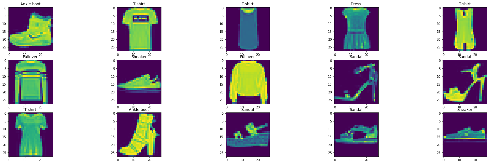
The dataset consists of 28x28 grayscale images and labels of range [0, 9] from 10 classes: T-shirt, trouser, pullover, dress, coat, sandal, shirt, sneaker, bag and ankle boot.

In order for the images to be usable by PyTorch, we have to convert them to torch.Tensor objects. Also, data normalisation improves overall performance. We will apply both operations, conversion and normalisation, to the datasets using torchvision.transforms and feed these ops to torchvision.datasets:

transform = torchvision.transforms.Compose(
    [
        torchvision.transforms.ToTensor(),
        torchvision.transforms.Normalize((0.5,), (0.5,)),
    ]
)

train_dataset = torchvision.datasets.FashionMNIST(
    "~/.torch/datasets", transform=transform, download=True, train=True
)

test_dataset = torchvision.datasets.FashionMNIST(
    "~/.torch/datasets", transform=transform, download=True, train=False
)

classes = (
    "T-shirt",
    "Trouser",
    "Pullover",
    "Dress",
    "Coat",
    "Sandal",
    "Shirt",
    "Sneaker",
    "Bag",
    "Ankle boot",
)

With the following method, we can visualise and save a sample of these images and their associated labels:

plt.figure(figsize=(30, 15))
for i, (image, label) in enumerate(train_dataset):
    if i == 15:
        break
    image = (image / 2 + 0.5).numpy()  # reverse transformation
    ax = plt.subplot(5, 5, i + 1)
    ax.set_title(classes[label])
    plt.imshow(image[0])

plt.savefig("sample_images.png")

PopTorch DataLoader

We can feed batches of data into a PyTorch model by simply passing the input tensors. However, this is unlikely to be efficient and can result in data loading being a bottleneck to the model, slowing down the training process. In order to make data loading easier and more efficient, there’s the torch.utils.data.DataLoader class, which is an iterable over a dataset and which can handle parallel data loading, a sampling strategy, shuffling, etc.

PopTorch offers an extension of this class with its poptorch.DataLoader class, specialised for the way the underlying PopART framework handles batching of data. We will use this class later in the tutorial, as soon as we have a model ready for training.

Build the model

We will build a simple CNN model for a classification task. To do so, we can simply use PyTorch’s API, including torch.nn.Module. The difference from what we’re used to with pure PyTorch is the loss computation, which has to be part of the forward function. This is to ensure the loss is computed on the IPU and not on the CPU, and to give us as much flexibility as possible when designing more complex loss functions.

class ClassificationModel(nn.Module):
    def __init__(self):
        super().__init__()
        self.conv1 = nn.Conv2d(1, 5, 3)
        self.pool = nn.MaxPool2d(2, 2)
        self.conv2 = nn.Conv2d(5, 12, 5)
        self.norm = nn.GroupNorm(3, 12)
        self.fc1 = nn.Linear(972, 100)
        self.relu = nn.ReLU()
        self.fc2 = nn.Linear(100, 10)
        self.log_softmax = nn.LogSoftmax(dim=1)
        self.loss = nn.NLLLoss()

    def forward(self, x, labels=None):
        x = self.pool(self.relu(self.conv1(x)))
        x = self.norm(self.relu(self.conv2(x)))
        x = torch.flatten(x, start_dim=1)
        x = self.relu(self.fc1(x))
        x = self.log_softmax(self.fc2(x))
        # The model is responsible for the calculation
        # of the loss when using an IPU. We do it this way:
        if self.training:
            return x, self.loss(x, labels)
        return x


model = ClassificationModel()
model.train()

ClassificationModel(
  (conv1): Conv2d(1, 5, kernel_size=(3, 3), stride=(1, 1))
  (pool): MaxPool2d(kernel_size=2, stride=2, padding=0, dilation=1, ceil_mode=False)
  (conv2): Conv2d(5, 12, kernel_size=(5, 5), stride=(1, 1))
  (norm): GroupNorm(3, 12, eps=1e-05, affine=True)
  (fc1): Linear(in_features=972, out_features=100, bias=True)
  (relu): ReLU()
  (fc2): Linear(in_features=100, out_features=10, bias=True)
  (log_softmax): LogSoftmax(dim=1)
  (loss): NLLLoss()
)

NOTE: self.training is inherited from torch.nn.Module which initialises its value to True. Use model.eval() to set it to False and model.train() to switch it back to True.

Prepare training for IPUs

The compilation and execution on the IPU can be controlled using poptorch.Options. These options are used by PopTorch’s wrappers such as poptorch.DataLoader and poptorch.trainingModel.

opts = poptorch.Options()

train_dataloader = poptorch.DataLoader(
    opts, train_dataset, batch_size=16, shuffle=True, num_workers=20
)

Train the model

We will need another component in order to train our model: an optimiser. Its role is to apply the computed gradients to the model’s weights to optimize (usually, minimize) the loss function using a specific algorithm. PopTorch currently provides classes which inherit from multiple native PyTorch optimisation functions: SGD, Adam, AdamW, LAMB and RMSprop. These optimisers provide several advantages over native PyTorch versions. They embed constant attributes to save performance and memory, and allow you to specify additional parameters such as loss/velocity scaling.

We will use SGD as it’s a very popular algorithm and is appropriate for this classification task.

optimizer = poptorch.optim.SGD(model.parameters(), lr=0.001, momentum=0.9)

We now introduce the poptorch.trainingModel wrapper, which will handle the training. It takes an instance of torch.nn.Module, such as our custom model, an instance of poptorch.Options which we have instantiated previously, and an optimizer. This wrapper will trigger the compilation of our model, using TorchScript, and manage its translation to a program the IPU can run. Let’s use it.

poptorch_model = poptorch.trainingModel(model, options=opts, optimizer=optimizer)

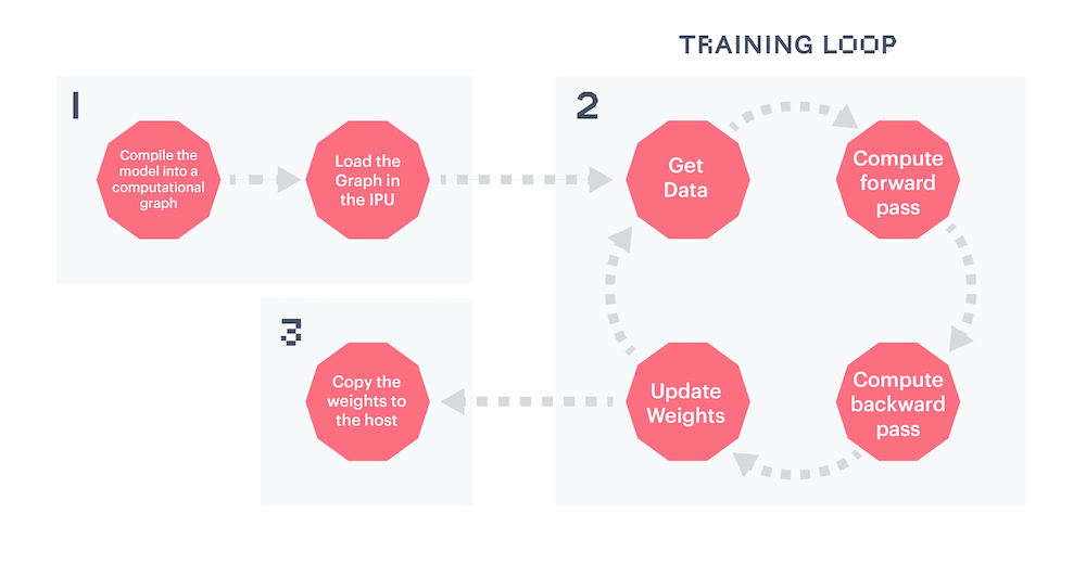
Training loop

Looping through the training data, running the forward and backward passes, and updating the weights constitute the process we refer to as the “training loop”. Graphcore’s Poplar graph program framework uses several optimisations to accelerate the training loop. Central to this is the desire to minimise interactions between the device (the IPU) and the host (the CPU), allowing the training loop to run on the device independently from the host. To achieve that virtual independence, Poplar creates a static computational graph and data streams which are loaded to the IPU, and then signals the IPU to get started until there’s no data left or until the host sends a signal to stop the loop.

The compilation, which transforms our PyTorch model into a computational graph and our dataloader into data streams, happens at the first call of a poptorch.trainingModel. The IPUs to which the graph will be uploaded are selected automatically during this first call, by default. The training loop can then start.

Once the loop has started, Poplar’s main task is to feed the data into the streams and to signal when we are done with the loop. The last step will then be to copy the final graph, meaning the model, back to the CPU - a step that PopTorch manages itself.

epochs = 5
for epoch in tqdm(range(epochs), desc="epochs"):
    total_loss = 0.0
    for data, labels in tqdm(train_dataloader, desc="batches", leave=False):
        output, loss = poptorch_model(data, labels)
        total_loss += loss

The model is now trained! There’s no need to retrieve the weights from the device as you would by calling model.cpu() with PyTorch. PopTorch has managed that step for us. We can now save and evaluate the model.

Use the same IPU for training and inference

After the model has been attached to the IPU and compiled after the first call to the PopTorch model, it can be detached from the device. This allows PopTorch to use a single device for training and inference (described below), rather than using 2 IPUs (one for training and one for inference) when the device is not detached. When using a POD system, detaching from the device will be necessary when using a non-reconfigurable partition.

poptorch_model.detachFromDevice()

Save the trained model

We can simply use PyTorch’s API to save a model in a .pth file, with the original instance of ClassificationModel and not the wrapped model.

Do not hesitate to experiment with different models: the model provided in this tutorial is saved in the static folder if you need it.

torch.save(model.state_dict(), "classifier.pth")

Evaluate the model

The model can be evaluated on a CPU but it is a good idea to use the IPU - since IPUs are blazing fast!

Evaluating your model on a CPU is slow if the test dataset is large and/or the model is complex.

Since we have detached our model from its training device, the device is now free again and we can use it for the evaluation stage.

The steps taken below to define the model for evaluation essentially allow it to run in inference mode. Therefore, you can follow the same steps to use the model to make predictions once it has been deployed.

model = model.eval()

To evaluate the model on the IPU, we will use the poptorch.inferenceModel class, which has a similar API to poptorch.trainingModel except that it doesn’t need an optimizer, allowing evaluation of the model without calculating gradients.

poptorch_model_inf = poptorch.inferenceModel(model, options=opts)

Then we can instantiate a new PopTorch Dataloader object as before in order to efficiently batch our test dataset.

test_dataloader = poptorch.DataLoader(opts, test_dataset, batch_size=32, num_workers=10)

This short loop over the test dataset is effectively all that is needed to run the model and generate some predictions. When running the model in inference mode, we can stop here and use the predictions as needed.

For evaluation, we can use the standard classification metrics from scikit-learn to understand how well our model is performing. This usually takes a list of labels and a list of predictions as the input, both in the same order. Let’s make both lists, and run our model in inference mode.

predictions, labels = [], []
for data, label in test_dataloader:
    predictions += poptorch_model_inf(data).data.max(dim=1).indices
    labels += label

Release IPU resources again:

poptorch_model_inf.detachFromDevice()

A simple and widely-used performance metric for classification models is the accuracy score, which simply counts how many predictions were right. But this metric alone isn’t enough. For example, it doesn’t tell us how the model performs with regard to the different classes in our data. We will therefore use another popular metric: a confusion matrix, which indicates how much our model confuses one class for another.

from sklearn.metrics import accuracy_score, confusion_matrix, ConfusionMatrixDisplay

print(f"Eval accuracy: {100 * accuracy_score(labels, predictions):.2f}%")
cm = confusion_matrix(labels, predictions)
cm_plot = ConfusionMatrixDisplay(cm, display_labels=classes).plot(
    xticks_rotation="vertical"
)

Eval accuracy: 89.25%

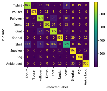
As you can see, although we’ve got an accuracy score of ~89%, the model’s performance across the different classes isn’t equal. Trousers are very well classified, with more than 96-97% accuracy whereas shirts are harder to classify with less than 60% accuracy, and it seems they often get confused with T-shirts, pullovers and coats. So, some work is still required here to improve your model for all the classes!

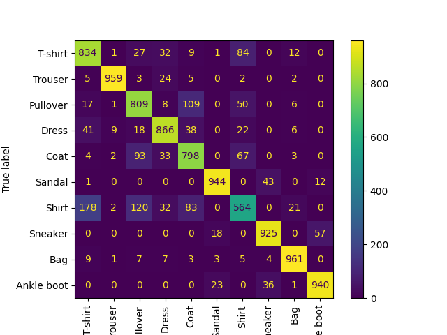
We can save this visualisation of the confusion matrix. Don’t hesitate to experiment: you can then compare your confusion matrix with the visualisation provided in the static folder.

cm_plot.figure_.savefig("confusion_matrix.png")

Using the model on our own images to get predictions

Now that we have a trained model which has also been validated, we can now use the model on arbitrary images which are not part of the FashionMNIST dataset. In this section we will use an image downloaded from the internet and predict the class of it.

Running our model on the IPU

We can then instantiate our model and load its state_dict which we saved earlier. We need to make sure that the model is then set to evaluation mode. We can then wrap our model with the PopTorch inference model which will let us run it on the IPU.

model = ClassificationModel()
model.load_state_dict(torch.load("classifier.pth"))
model.eval()

poptorch_model = poptorch.inferenceModel(model, options=poptorch.Options())

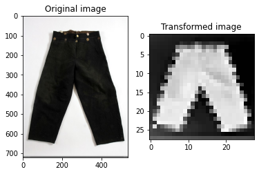
Next we can load our image into our Python program. To do this we will use the Python Imaging Library (PIL) by supplying our image as a path. To get our image ready for evaluation, we need to make sure that the image is in the same ‘format’ as the images which were in the FashionMNIST dataset. This means that we need to resize our image to 28x28 pixels and make it grayscale.

Note: We can download images on a remote machine using wget: wget "https://bit.ly/3uKBBDS" -O ./images/trousers.jpg

Image attribution: Elisabeth Eriksson / Nordiska museet, CC BY 4.0 https://creativecommons.org/licenses/by/4.0, via Wikimedia Commons

from PIL import Image, ImageOps

img = Image.open("images/trousers.jpg").resize((28, 28))
img = ImageOps.grayscale(img)

Another factor we have to consider is that all of the images in the FashionMNIST dataset have a black background. This means that if our image’s background is light, then the model will incorrectly classify the image (another limitation due to our simple model). We can get around this by checking the pixel value in one corner of the image and if it’s light, then invert the whole image. Afterwards we can transform our image into a tensor which can be fed into the model.

if img.getpixel((1, 1)) > 200:
    img = ImageOps.invert(img)

transform = torchvision.transforms.Compose(
    [
        torchvision.transforms.ToTensor(),
        torchvision.transforms.Normalize((0.5,), (0.5,)),
    ]
)

img_tensor = transform(img)

We can visualise our original image before and after the transformations:

f, ax = plt.subplots(1, 2)
ax[0].imshow(Image.open("images/trousers.jpg"))
ax[0].set_title("Original image")
img_transform = torchvision.transforms.ToPILImage()
ax[1].imshow((img_transform(img_tensor)).convert("RGBA"))
ax[1].set_title("Transformed image")

plt.savefig("image_before_after.png")

The model expects a four-dimensional tensor with the dimensions corresponding respectively to: batch size, number of colour channels, and the height and width of the image. Since we have a single image represented as a three-dimensional tensor, we expand it to include a batch dimension using the unsqueeze function.

The output from the model will be a tensor consisting of 10 values (one for each class). The highest value within the tensor will be the piece of clothing which the model predicts our image to be.

img_tensor = img_tensor.unsqueeze(0)

output = poptorch_model(img_tensor)
print(output)

Graph compilation: 100%|██████████| 100/100 [00:09<00:00]
tensor([[-4.4716, -0.9097, -3.2780, -5.8899, -3.4709, -1.4561, -1.8613, -6.6171,
         -2.1167, -5.5265]])

Now we interpret the output and print the name of the class.

prediction_idx = int(output.argmax())

poptorch_model.detachFromDevice()

print("IPU predicted class:", classes[prediction_idx])

IPU predicted class: Trouser

Running our model on the CPU

If you wanted to use the model on a different machine, perhaps not the IPU, then you can import the classification model and the tuple of classes from earlier. This would mean that you can run the prediction without having to import PopTorch at all and we would just need the .pth model file.

model = ClassificationModel()
model.load_state_dict(torch.load("classifier.pth"))
model.eval()

output = model(img_tensor)
print("CPU predicted class:", classes[int(output.argmax())])

CPU predicted class: Trouser

Limitations with our model

Due to the small size of the training dataset and low complexity of the model, there are many limitations with our model. The examples need to be carefully selected to match the distribution of the training dataset, otherwise our model may classify incorrectly.

The following need to be considered when choosing images for classification:

• The orientation of the piece of clothing must be horizontal,

• The background of the image must be a solid colour,

• The piece of clothing is photographed on its own; it cannot be worn by a person.

Doing more with poptorch.Options

This class encapsulates the options that PopTorch and PopART will use alongside our model. Some concepts, such as “batch per iteration” are specific to the functioning of the IPU, and within this class some calculations are made to reduce risks of errors and make it easier for PyTorch users to use IPUs.

The list of these options is available in the documentation. We introduce here four of these options so you get an idea of what they cover.

deviceIterations

Remember the training loop we have discussed previously. A device iteration is one cycle of that loop, which runs entirely on the IPU (the device), and which starts with a new batch of data. This option specifies the number of batches that is prepared by the host (CPU) for the IPU. The higher this number, the less the IPU has to interact with the CPU, for example to request and wait for data, so that the IPU can loop faster. However, the user will have to wait for the IPU to complete all iterations before getting the results back. The maximum number of iterations is the total number of batches in your dataset, and the default value is 1.

replicationFactor

This is the number of replicas of a model. A replica is a copy of the same model on multiple devices. We use replicas as an implementation of data parallelism, where the same model is served with several batches of data at the same time but on different devices, so that the gradients can be pooled. To achieve the same behaviour in pure PyTorch, you’d wrap your model with torch.nn.DataParallel, but with PopTorch, this is an option. Of course, each replica requires one IPU. So, if the replicationFactor is two, two IPUs are required.

randomSeed

An advantage of the IPU architecture is an on-device pseudo-random number generator (PRNG). This option sets both the seed for the PRNG on the IPU and PyTorch’s seed, which is usually set using torch.manual_seed.

useIpuModel

An IPU Model is a simulation, running on a CPU, of an actual IPU. This can be helpful if you’re working in an environment where no IPUs are available but still need to make progress on your code. However, the IPU Model doesn’t fully support replicated graphs and its numerical results can be slightly different from what you would get with an actual IPU. You can learn more about the IPU Model and its limitations with our documentation.

How to set the options

These options are callable, and can be chained as they return the instance. One can therefore do the following:

opts = (
    poptorch.Options()
    .deviceIterations(20)
    .replicationFactor(2)
    .randomSeed(123)
    .useIpuModel(True)
)

Summary

In this tutorial, we started learning about PopTorch and how to use it to create and train a model which we then be used for inference. We used Torchvision to load the FashionMNIST dataset, a more complex alternative to the well-known MNIST dataset. We created a classification model and trained it on a training subset of our dataset by feeding the images into our model using the PopTorch DataLoader class. After training, we evaluated our model using the testing dataset to measure a metric for our model. Lastly, we used the trained model to predict the class of clothing for our own images, which the model had never seen before. When submitting our own images for classification, we needed to make sure that we were aware of the limitations of our model.

Next steps:

To continue learning about PopTorch and how to use it to run your models on the IPU, look at our tutorials on efficient data loading, pipelining your model in PopTorch and fine-tuning a BERT model to run on the IPU.

Generated:2022-09-27T15:24 Source:walkthrough.py SDK:3.0.0+1145 SST:0.0.8